This document discusses relative valuation, which values an asset based on comparable assets currently priced in the market. It outlines the steps in relative valuation, including analyzing the subject company, selecting comparable companies, choosing valuation multiples, calculating multiples for comparables, and valuing the subject company. It also discusses various valuation multiples used in relative valuation like P/E, P/B, P/S, EV/EBITDA, and their fundamental determinants. Best practices for using multiples are also presented.

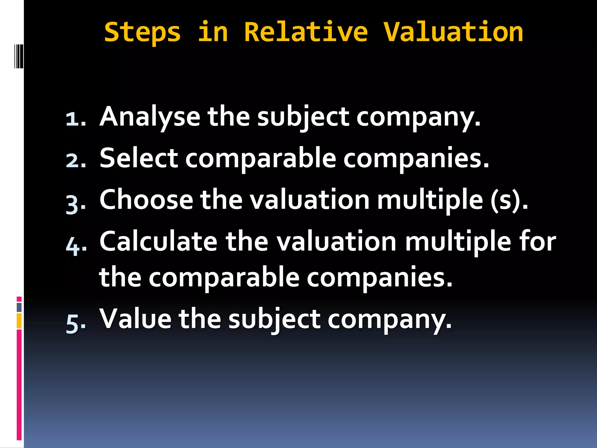
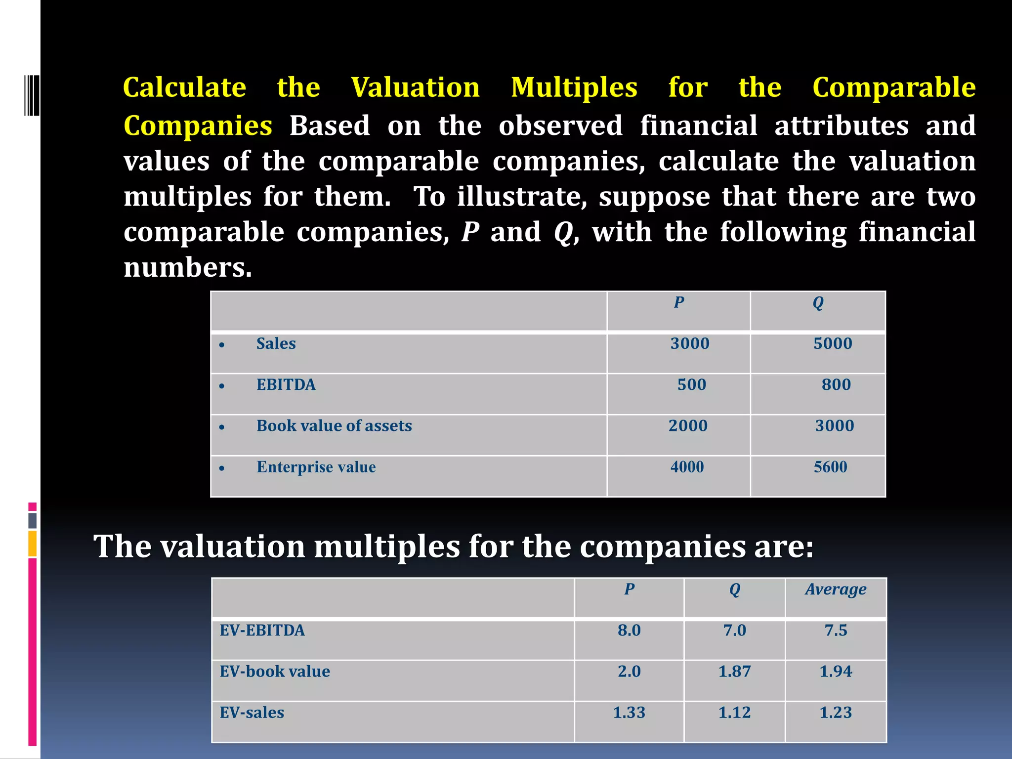
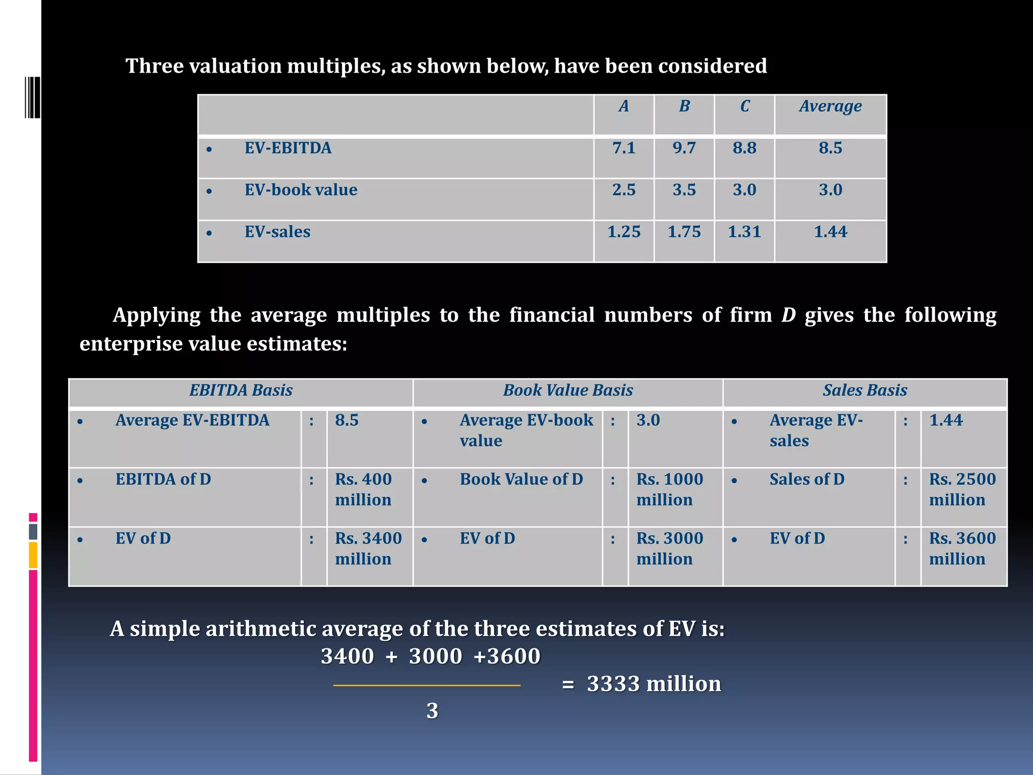
1. Chapter5
RelativeValuation

2. Outline
 Steps Involved in RelativeValuation
 EquityValuation Multiples
 EnterpriseValuation Multiples
 Choice of Multiple
 Best Practices Using Multiples
 Assessment of RelativeValuation

3. Introduction
In DCF valuation, an asset is valued on the
basis of its cash flow, growth, and risk
characteristics. In relative valuation, an
asset is valued on the basis of how similar
assets are currently priced in the market.
As Dan Ariely put it: “Everything is relative
even when it shouldn’t be. Humans rarely
choose in ‘absolute terms.’ We don’t have an
internal meter that tells us how much
things are worth. Rather, we focus on the
relative advantage of one thing over
another, and estimate value accordingly.”

4. Introduction
Common sense and economic logic tell us that similar assets
should sell at similar prices. Based on this principle, one can value
an asset by looking at the price at which a comparable asset has
changed hands between a reasonably informed buyer and a
reasonably informed seller. For example, if you want to sell your
residential flat, you can estimate its appropriate asking price by
looking at market comparables. Suppose your flat measures 2000
square feet and recently a flat in the neighbourhood measuring
1500 square feet sold for Rs.4,500,000 (at the rate of Rs.3,000 per
square feet). As a first pass, you can put a value of 2000 X Rs. 3000
= Rs.6,000,000 for your flat.
Relative valuation is often considered as a substitute for DCF
valuation. However, as our discussion in this chapter shows, the
DCF approach provides the conceptual foundation for most relative
valuation metrics. Hence the two approaches should be seen as
complementary.

5. Steps in Relative Valuation
1. Analyse the subject company.
2. Select comparable companies.
3. Choose the valuation multiple (s).
4. Calculate the valuation multiple for
the comparable companies.
5. Value the subject company.

6. 1. Analyse the Subject Company To begin with, an in-depth
analysis of the competitive and financial position of the
subject company (the company to be valued) must be
conducted. The key aspects to be covered in this
analysis are as follows:
 Product portfolio and market segments covered by the
firm
 Availability and cost of inputs
 Technological and production capability
 Market image, distribution reach, and customer loyalty
 Product differentiation and economic cost position
 Managerial competence and drive
 Quality of human resources
 Competitive dynamics
 Liquidity, leverage, and access to funds
 Turnover, margins, and return on investment.

7. 2. Select Comparable Companies
 Often, it is hard to find truly comparable
companies.
 Look at 10 to 15 companies in the same
industry and select at least 3 to 4 which come
‘as close as possible.’

8. 3. Choose the Valuation
Multiple (s)
EquityValuation Multiples
 Price – earnings ratio
 Price – book value ratio
 Price – sales ratio
EnterpriseValuation Multiples
 EV – EBITDA ratio
 EV – FCFF ratio
 EV – book value ratio
 EV – sales ratio

9. Calculate the Valuation Multiples for the Comparable
Companies Based on the observed financial attributes and
values of the comparable companies, calculate the valuation
multiples for them. To illustrate, suppose that there are two
comparable companies, P and Q, with the following financial
numbers.
The valuation multiples for the companies are:
P Q
 Sales 3000 5000
 EBITDA 500 800
 Book value of assets 2000 3000
 Enterprise value 4000 5600
P Q Average
EV-EBITDA 8.0 7.0 7.5
EV-book value 2.0 1.87 1.94
EV-sales 1.33 1.12 1.23

10. Value the Subject Company
Given the observed valuation multiples of the
comparable companies, the subject company may be
valued. A simple way to do is to apply the average
multiples of the comparable companies to the relevant
financial attributes of the subject company and obtain
several estimates (as many as the number of valuation
multiples used) of enterprise value for the subject
company and then take their arithmetic average.
A more sophisticated way to do is to look at how
the growth prospects, risk characteristics, and size of
the subject company (the most important drivers of
valuation multiples) compare with those of
comparable companies and then take a judgmental
view of the multiples applicable to it.

11. Illustration
The following financial information is available for company D, an
unlisted pharmaceutical company, which is being valued.
 EBITDA : Rs. 400 million
 Book value of assets : Rs. 1,000 million
 Sales : Rs. 2,500 million
Based on an evaluation of a number of listed pharmaceutical
companies, A, B, and C have been found to be comparable to
company D. The financial information for these companies is
given below:
A B C
 Sales 1600 2000 3200
 EBITDA 280 360 480
 Book value of assets 800 1000 1400
 Enterprise value (EV) 2000 3500 4200

12. Three valuation multiples, as shown below, have been considered
Applying the average multiples to the financial numbers of firm D gives the following
enterprise value estimates:
A simple arithmetic average of the three estimates of EV is:
3400 + 3000 +3600
= 3333 million
3
A B C Average
 EV-EBITDA 7.1 9.7 8.8 8.5
 EV-book value 2.5 3.5 3.0 3.0
 EV-sales 1.25 1.75 1.31 1.44
EBITDA Basis Book Value Basis Sales Basis
 Average EV-EBITDA : 8.5  Average EV-book
value
: 3.0  Average EV-
sales
: 1.44
 EBITDA of D : Rs. 400
million
 Book Value of D : Rs. 1000
million
 Sales of D : Rs. 2500
million
 EV of D : Rs. 3400
million
 EV of D : Rs. 3000
million
 EV of D : Rs. 3600
million

13. P/E Ratio
 Marketing price per share /
Earnings per share

14. Fundamental Determinants
From a fundamental point of view
(1 - b)
Po/E1 =
r – ROE X b
where (1 - b) is the dividend payout ratio, r is the cost of equity, ROE
is the return on equity, and b is the ploughback ratio.
Example Alpha Company’s ROE is 18 percent and its r is 15 percent.
Alpha’s dividend payout ratio is 0.4 and its ploughback ratio 0.6. So,
from a fundamental point of view, Alpha’s P/E multiple is:
0.4
Po/E1 = = 9.52
0.15 – 018 X 0.6

15. Drawbacks of P/E
 Negative EPS
 Maintainable EPS
 Manipulation

16. P/B Ratio
Shareholders’ funds – Preference Capital
Number of outstanding equity shares

17. Fundamental Determinants
From a fundamental point of view,
Po ROE (1 - b)
=
BVo r – g
where ROE is the return on equity, g is the growth rate, (1 - b) is the
dividend payout ratio, and r is the rate of return required by equity
investors.
Example Magna Corporation’s ROE is 20 percent and its r is 16 percent.
Magna’s dividend payout ratio is 0.4 and its g is 12 percent. From a
fundamental point of view, Magna’s.
Po 0.20 (0.4)
= = 2.00
BVo 0.16 – 0.12

18. Drawbacks of P/B
 Intangible assets
 Inflation and technological changes
 Different business models

19. P/S Ratio
 Rationale
 Norm

20. Fundamental Determinants
From a fundamental point of view,
Po NPM (1+ g) (1 - b)
=
So r – g
where NPM is the net profit margin ratio, g is the growth rate, (1 - b) is
the dividend payout ratio, and r is the rate of return required by
equity investors.
Example Black Limited has a NPM of 8 percent and a growth rate 12
percent. Black’s dividend payout ratio (1 - b) is 0.3 and its r is 0.16.
from a fundamental point of view, Black’s
Po 0.08(1.12) (0.3)
= = 0.67
So 0.16 – 0.12

21. Reasons for P/S
 No manipulation
 Always positive
 More stable than EPS
 PS ratio .. long-term average
returns

22. Summation
Let us look at the equations for PE ratio, PBV ratio, and PS ratio.
(1-b) = (1-b)
PE =
r – ROE x b r – g
ROE (1-b)
PBV =
(r – g)
NPM (1+g) (1-b)
PS =
r - g
Looking at these equations, we find that there is one variable that
dominates when it comes to explaining each multiple – it is g for PE, ROE
for PBV, and NPM for PS. This variable – the dominant explanatory
variable – is called the companion variable.

23. Companion Variables &
Modified Multiples
Taking into account the importance of the
companion variable, investment practitioners
often use modified multiples which are defined
below.
PE to growth multiple, referred to as PEG : PE
g
PBV to ROE, referred to as value ratio : PBV
ROE
PS to NPM, referred to as PSM : PS
Net profit margin

24. EV to EBITDA Ratio
 EV
EBITDA

25. Fundamental Determinants
EV ROIC – g
= X (1 - DA) (1 - t)
EBITDA ROIC X (WACC – g)
where ROIC is the return on invested capital, g
is the growth rate, DA is the depreciation and
amortisation charges as a percent of EBITDA, t
is the tax rate, and WACC is the weighted
average cost of capital.

26. Determinants of EV/EBITDA
g
EVo = ICo x ROIC x 1 -
ROIC
ROIC - g
= IC o x
WACC - g
EV IC o ROIC – g
= x
EBITDA EBITDA WACC – g
EBITDA = NOPLAT / (1 - DA) (1 - t)
EV ICo ROIC – g
= x
EBITDA NOPLAT / (1 - DA) (1 - t) WACC - g
EV ROIC – g
= x (1 - DA) (1 - t)
EBITDA ROIC x (WACC - g)

27. EV/EBIT Multiple
EV
EBIT
EV
EBIT (1 -Tax)

28. Fundamental Determinants
EVo (1 - t) (1 – Reinvestment rate)
=
EBIT1 WACC - g
where t is the tax rate, WACC is the weighted
average cost of capital, and g is the growth rate.

29. EV/FCFF Multiple
EV
FCFF

30. Fundamentals Determinants
EVo 1
=
FFCF1 WACC - g
where WACC is the weighted average cost of
capital and g is the growth rate.

31. EV/BV
EV
BV

32. Fundamental Determinants
EVo ROIC - g
=
BVo WACC - g
where ROIC is the return on invested capital, g
is the growth rate, and WACC is the weighted
average cost of capital.

33. Example
Example Felix Company has an ROIC of 15
percent, g of 10 percent, and WACC of 12
percent. From a fundamental point of view
Felix’s:
EVo 0.15 -0.10
= = 1.67
BVo 0.12 – 0.10

34. Fundamental Determinants
EVo After-tax operating margin (1 + g)
(1 – Reinvestment rate)
=
So WACC - g
where g is the growth rate and WACC is the
weighted average cost of capital.

35. Determinants of EV/Sales
EBITo (1 + g) (1 - t) (1 – Reinvestment rate)
EVo =
WACC – g
EVo EBIT (1 + g) (1 - t) (1 – Reinvestment rate)
S0
=
So WACC – g
After-tax operating margin (1 + g)
(1 – Reinvestment rate)
=
WACC - g

36. Operational Multiples
An operational multiple expresses the enterprise
value (EV) in relation to a specific operational
variable, which is usually a key driver of revenue
or cash flow. Some examples of operational
multiples from different industries are shown
below:
Industry Operational Multiple
Energy EV/KWH production capacity
Hotel EV/Number of rooms
Media EV/Number of subscribers
Telecommunications EV/Number of subscribers

37. From a fundamental point of view, the general
formula for an operational multiple is:
EV ROIC – g NOPLAT
= X
Unit ROIC X (WACC -g) Unit
where ROIC is the return on invested capital,
g is the growth rate, WACC is the weighted
average cost of capital, NOPLAT is the net
operating profit less adjusted taxes, and unit
is the measure of the operational variable.

38. Three Ways to Find the Best
Multiple
 Fundamental Approach
 Statistical Approach
 Conventional Approach

39. Most Commonly Used Multiples
P/E : Proven track record of earnings and no
significant non-cash expenses.
PEG : Stable EPS growth rates and risk
characteristics
P/B : Balance sheets reflect well market values
(Financial institutions)
EV/EBITDA : Substantial non-cash expenses
(Airlines,Telecom operators)
EV/FCFF : Stable growth and predictable capex.
EV/Sales : Young firms .. - earnings

40. Best Practices Using Multiples
A judicious use of multiples can provide valuable
insights, whereas an unthinking application of
multiples can result in confusion and distortion.
Bear in mind the following best practices with
respect to multiples:
 Define multiples consistently.
 Choose comparables with similar profitability
and growth prospects.
 Identify the fundamental determinants.
 Use multiples that use forward-looking
estimates.
 Prefer enterprise-value multiples.

41. Emphasis on Relative
Valuation in Practice
 Investment rules of thumb are .. In terms of
multiples.
 Even when DCF valuation is used; the
recommendations are usually based on
valuation multiple (s).
 Multiples serve as a convenient shorthand for
communication and provide a useful check on
valuation.
 Multiples are easier to sell as well as defend.

42. Weaknesses of Relative
Valuation
 Greater scope for manipulation.
 Reflect valuation errors of the
market .

43. Reconciling Relative and
DCF Valuation
 DCF valuation and relative valuation generally
produce different estimates of value.
 Main reason.. different views of market efficiency.
(or inefficiency).
 DCF valuation assumes that the markets make
mistakes (which may apply to the entire market or
parts thereof) but correct these mistakes over
time.
 Relative valuation assumes that on average the
markets are correct, although they may make
mistakes on individual stocks.

44. MARKET TRANSACTION METHOD
A variant of the market comparable method, the market
transaction method employs transaction multiples in lieu of
trading multiples. As the name suggests, transaction
multiples are the multiples implicit in recent
acquisitions/disposals of similar companies.
The primary advantage of this method is that the transaction
multiples are based on negotiation between more informed
buyers and sellers and hence are less likely to be affected by
market inefficiencies. However, its limitations are that the
characteristics of recently transacted companies and the
conditions under which they may have been transacted are
likely to be very different. Further, the requisite information
relating to transactions, particularly when unlisted
companies are involved, may not be available.

45. While using transaction multiples, the following factors
should be considered: nature of transaction (friendly or
hostile), the prevailing market sentiment at the time of
transaction, form of compensation (stock or cash), contingent
payments (if any), and so on.

46. SUMMARY OF THE STEPS IN THE RELATIVE
VALUATION METHOD
1. Determine the criteria for selecting comparable publicly traded
companies.
2. Identify the companies that meet the criteria.
3. Decide on the relevant time period for comparative analysis.
4. Obtain the financial statements for the subject company and
comparable publicly limited companies for the time period
decided in Step 3, and make appropriate adjustments to the
same.
5. Compile the relevant financial ratios for the subject and
comparable companies.
6. Decide the value multiples to be used.
7. Obtain the market price for the equity stock for each comparable
company as of the valuation date. If the enterprise valuation
multiples are used, obtain the market value of all securities
included in the invested capital.
8. Compile the value multiple tables for all the comparable
companies.

47. SUMMARY OF THE STEPS IN THE RELATIVE
VALUATION METHOD
9. Analyse the value multiples of the comparable companies in
conjunction with the comparative financial analysis of the
subject company and comparable companies and decide on the
appropriate value of the multiples to be used for the subject
company.
10.Calculate the indicative value of the subject company according
to each value multiple, by multiplying the appropriate value of
the multiple with the relevant financial variable for the subject
company.
11.Obtain a weighted average of the indicative values determined in
Step 10 to get an estimate of “value as if publicly traded” (a
marketable, minority ownership interest value).
12.Adjust this value, if appropriate, for factors not reflected in the
value as if publicly traded, such as premium for control or
discount for lack of marketability.

48. Summary
 In relative valuation, an asset is valued on the basis of how similar
assets are currently priced in the market.
 The relative valuation of a company involves the following steps: (i)
analyse the subject company, (ii) select comparable companies, (iii)
choose the valuation multiple (s), (iv) calculate the valuation multiple(s)
for the comparable companies, and (v) value the subject company.
 The commonly used equity valuation multiples are: price-to-earnings
multiple, price-to-book value multiple, and price –to-sales multiple.
 The commonly used enterprise valuation (EV) multiples are: EV-FFCF-
ratio, EV-EBITDA multiple, EV-book value multiple, and EV-sales
multiple..
 Since different multiples produce different values, the choice of multiple
can make a big difference to your value estimate.
 In choosing the multiple the analyst can adopt the multiple that reflects
his bias (the cynical view), or use all the multiples (the bludgeon view),
or pick the “best” multiple.

49.  There are three ways to find the best multiple. The fundamental
approach suggests that we should use the variable that has the
highest correlation with the firms value. The statistical approach calls
for regressing each multiple against the fundamentals that
theoretically affect the value and using the multiple with the highest
R-squared. The conventional approach involves using the multiple
that has become the most commonly used one for a specific situation
or sector.
 The following are the best practices with respect to multiples: (a)
choose comparables with similar profitability and growth prospects. (b)
use multiples that use forward-looking estimates, (c) prefer enterprise-
value multiples.
 Relative valuation seems to be more popular compared to DCF
valuation because (a) it relies on multiples that are easy to relate to
and easy to obtain, and (b) it is easier to sell as well as defend.
 Notwithstanding its popularity, relative valuation suffers from certain
weakness. (a) it provides the analyst greater scope for valuation; (b)
the multiples used in relative valuation reflect the valuation errors
(overvaluation or undervaluation of the market).

50. THANK YOU