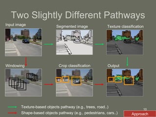
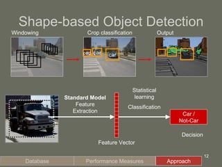
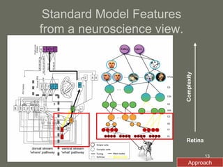
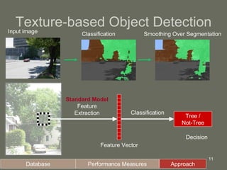
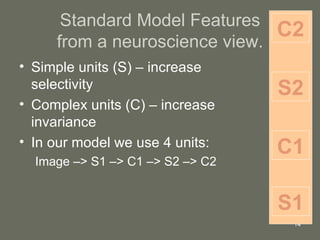
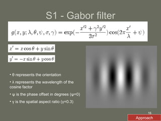
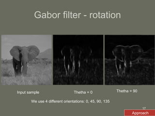
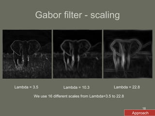
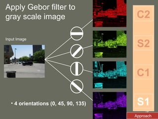
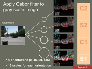
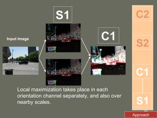
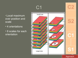
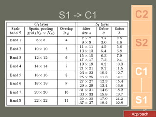
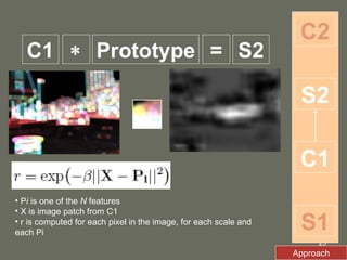
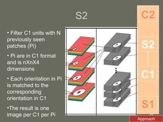
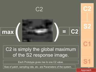
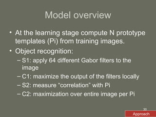
1. The document presents a framework for visual object recognition inspired by the visual cortex. It uses texture-based and shape-based pathways to recognize objects in complex scenes. 2. The model first applies Gabor filters to extract features, then uses complex cells to maximize responses locally. Simple cells then correlate the features with prototype templates before complex cells find the global maximum. 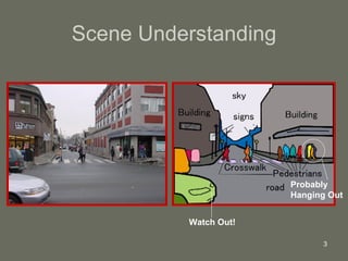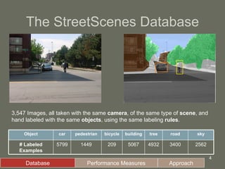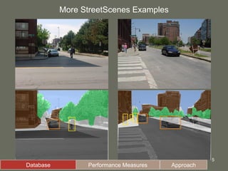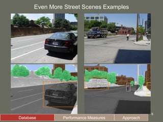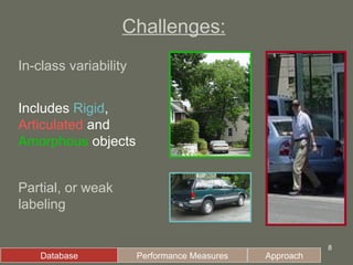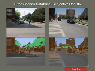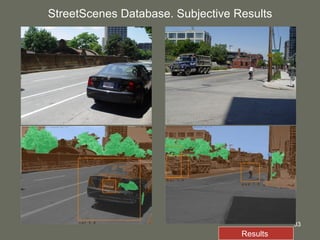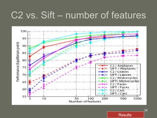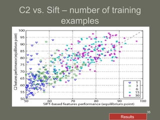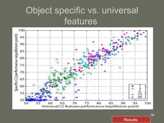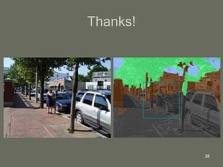3. The model is tested on a street scene image database, showing it can learn from fewer examples than SIFT features and outperforms using object-specific versus universal features.

1. Robust Object Recognition with Cortex-like Mechanisms (PAMI, 06) Presented by Ala Stolpnik T. Serre, L. Wolf, S. Bileschi, M. Riesenhuber, and T. Poggio

2. Introduction A general framework for the recognition of complex visual scenes The system follows the organization of visual cortex Texture and shape based object recognition

3. Scene Understanding Watch Out! Probably Hanging Out

4. The StreetScenes Database 3,547 Images, all taken with the same camera , of the same type of scene , and hand labeled with the same objects , using the same labeling rules . Database Performance Measures Approach sky road tree building bicycle pedestrian car Object 2562 3400 4932 5067 209 1449 5799 # Labeled Examples

5. More StreetScenes Examples Database Performance Measures Approach

6. Even More Street Scenes Examples Database Performance Measures Approach

7. Challenges: In-class variability Partial, or weak labeling Includes Rigid, Articulated and Amorphous objects Database Performance Measures Approach

8. Challenges: In-class variability Partial, or weak labeling Includes Rigid , Articulated and Amorphous objects Database Performance Measures Approach

9. Texture Sample Locations Building, Tree, Road and Sky Hand-drawn Labels Training Sample Locations Database Performance Measures Approach

10. Input image Segmented image Texture classification Windowing Crop classification Output Texture-based objects pathway (e.g., trees, road..) Shape-based objects pathway (e.g., pedestrians, cars..) car car ped Approach Two Slightly Different Pathways

11. Texture-based Object Detection Input image Classification Smoothing Over Segmentation Tree / Not-Tree Standard Model Feature Extraction Classification Database Performance Measures Approach Feature Vector Decision Feature Vector Decision

12. Shape-based Object Detection Windowing Crop classification Output car car ped Car / Not-Car Standard Model Feature Extraction Statistical learning Classification Database Performance Measures Approach Feature Vector Decision

13. Standard Model Features from a neuroscience view. Retina Complexity Approach

14. Standard Model Features from a neuroscience view. Simple units (S) – increase selectivity Complex units (C) – increase invariance In our model we use 4 units: Image –> S1 –> C1 –> S2 –> C2 C1 S2 C2 S1

15. Overview Introduction The model Results Approach

16. S1 - Gabor filter θ represents the orientation λ represents the wavelength of the cosine factor ψ is the phase offset in degrees (ψ=0) γ is the spatial aspect ratio (γ=0.3) Approach

17. Gabor filter - rotation Input sample Thetha = 0 Thetha = 90 Approach We use 4 different orientations: 0, 45, 90, 135

18. Gabor filter - scaling Lambda = 3.5 Lambda = 22.8 Lambda = 10.3 Approach We use 16 different scales from Lambda=3.5 to 22.8

19. S1 Input Image 4 orientations (0, 45, 90, 135) C1 S2 C2 Approach Apply Gebor filter to gray scale image

20. Apply Gebor filter to gray scale image Input Image S1 C1 S2 C2 Approach 4 orientations (0, 45, 90, 135) 16 scales for each orientation

21. S1 S1 C1 S2 C2 Approach 4 orientations 16 scales for each orientation Total: 64 S1 units

22. Input Image S1 C1 S1 C1 S2 C2 Local maximization takes place in each orientation channel separately, and also over nearby scales. Approach

23. C1 S1 C1 S2 C2 Approach Local maximum over position and scale 4 orientations 8 scales for each orientation

24. S1 -> C1 Approach S1 C1 S2 C2

25. S1 C1 S2 C2 Approach P i is one of the N features X is image patch from C1 r is computed for each pixel in the image, for each scale and each Pi C1 S2 Prototype  =

26. S2 Approach Filter C1 units with N previously seen patches (Pi) Pi are in C1 format and is nXnX4 dimensions Each orientation in Pi is matched to the corresponding orientation in C1 The result is one image per C1 per Pi S1 C1 S2 C2

27. C2 C2 is simply the global maximum of the S2 response image. S1 C1 S2 C2 Each Prototype gives rise to one C2 value. C2 = max ( ) Size of patch, sampling rate, etc. are Parameters of the system. Approach

28. Overview Make classification using SVM Approach

29. The learning stage Where do we get the Pi from? Input: a collection of images (Task specific of general dictionary) Each Pi is from nXnX4 dimensions. Where n can be 4, 8, 12, or 16. Pi selection: Select random image Convert the image to C1 Select nXn dimensional patch randomly from the C1 and this is our Pi Approach

30. Model overview At the learning stage compute N prototype templates (Pi) from training images. Object recognition: S1: apply 64 different Gabor filters to the image C1: maximize the output of the filters locally S2: measure “correlation” with Pi C2: maximization over entire image per Pi Approach

31. Overview Goals The model Results

32. StreetScenes Database. Subjective Results Results

33. StreetScenes Database. Subjective Results Results

34. C2 vs. Sift – number of features Results

35. C2 vs. Sift – number of training examples Results

36. Object specific vs. universal features Results

37. Conclusion A general framework for the recognition of complex visual scenes The system follows the organization of visual cortex Texture and shape based object recognition Capability of learning from only a few training examples

38. Thanks!