Download to read offline
![29
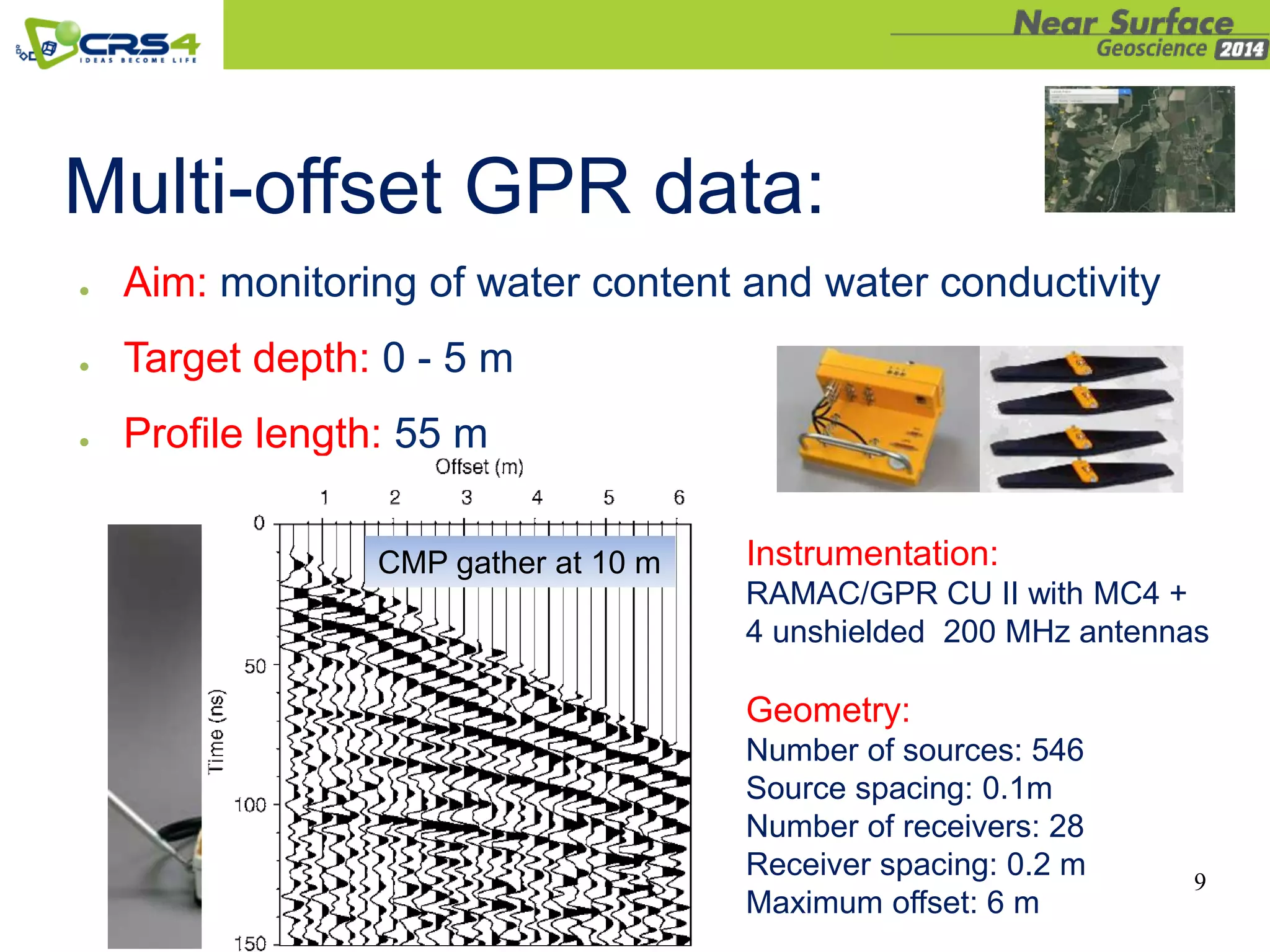
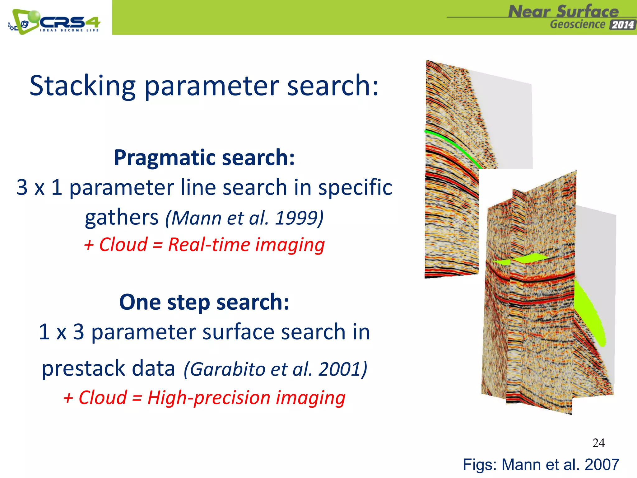
Some CMP gathers:
CMP 1171 CMP 1267CMP 1069
Offset [dm] Offset [dm] Offset [dm]
Time[ms]
Time[ms]
Time[ms]](https://image.slidesharecdn.com/nearsurface2014zhfinal-150724103113-lva1-app6891/75/Real-time-or-full-precision-CRS-imaging-using-a-cloud-computing-portal-multi-offset-GPR-and-SH-wave-examples-Zeno-Heilman-29-2048.jpg)
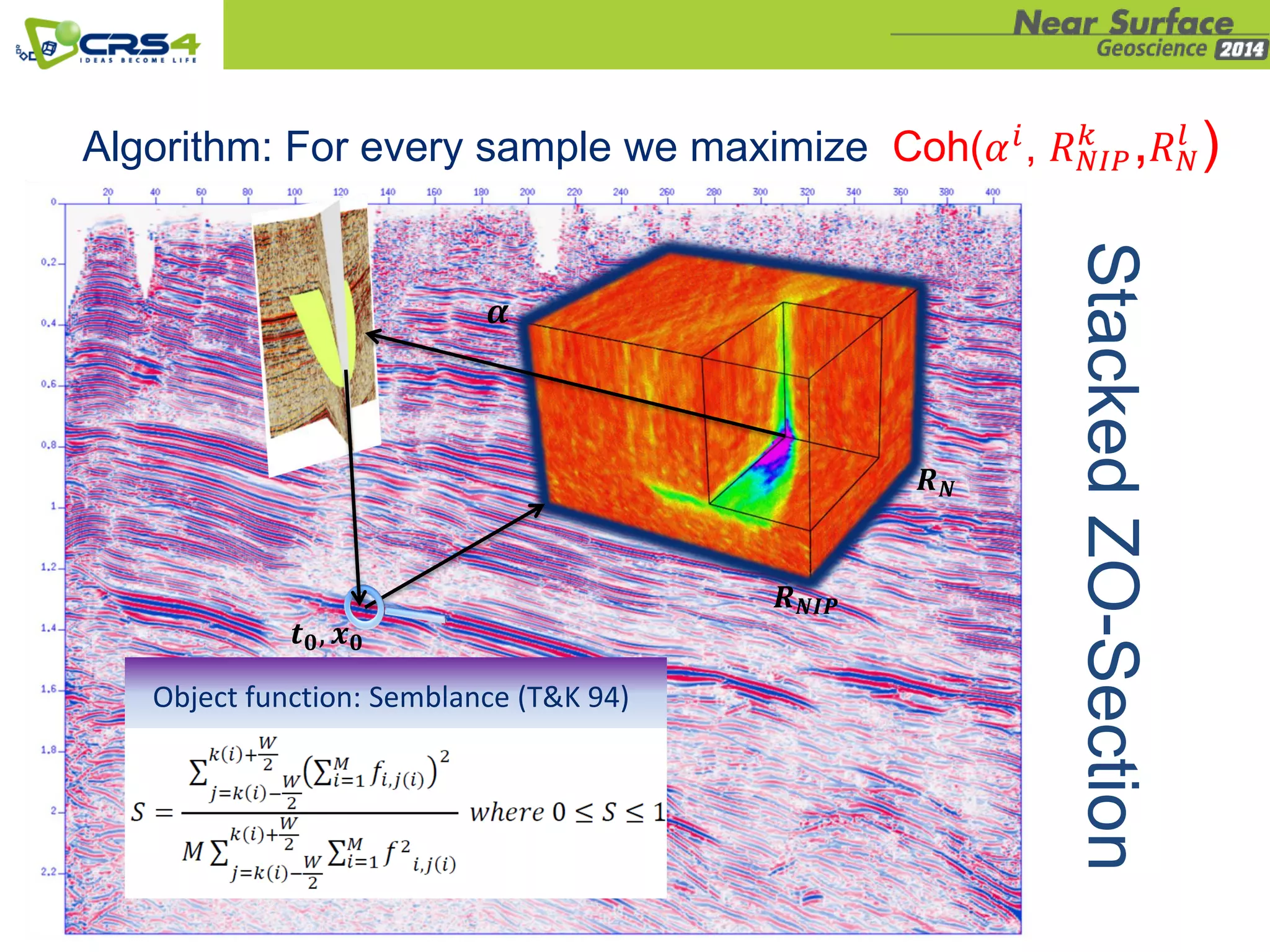
![Computational cost:
0 50 100
3x1 Parameter
2-Parameter
3-Parameter
submission-time
[min] on 30 CPU
runtime [min] on
30 CPUs](https://image.slidesharecdn.com/nearsurface2014zhfinal-150724103113-lva1-app6891/75/Real-time-or-full-precision-CRS-imaging-using-a-cloud-computing-portal-multi-offset-GPR-and-SH-wave-examples-Zeno-Heilman-33-2048.jpg)

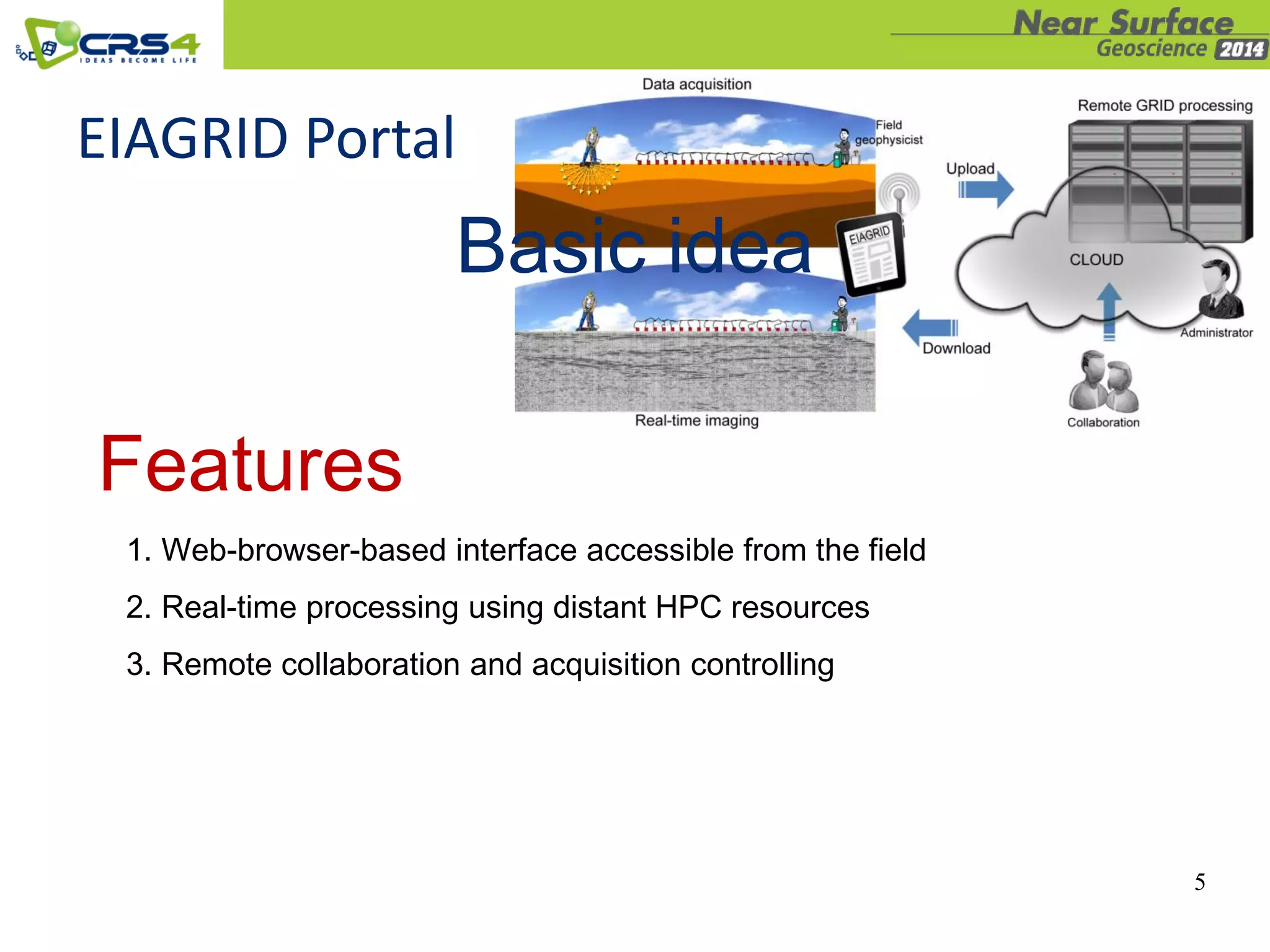
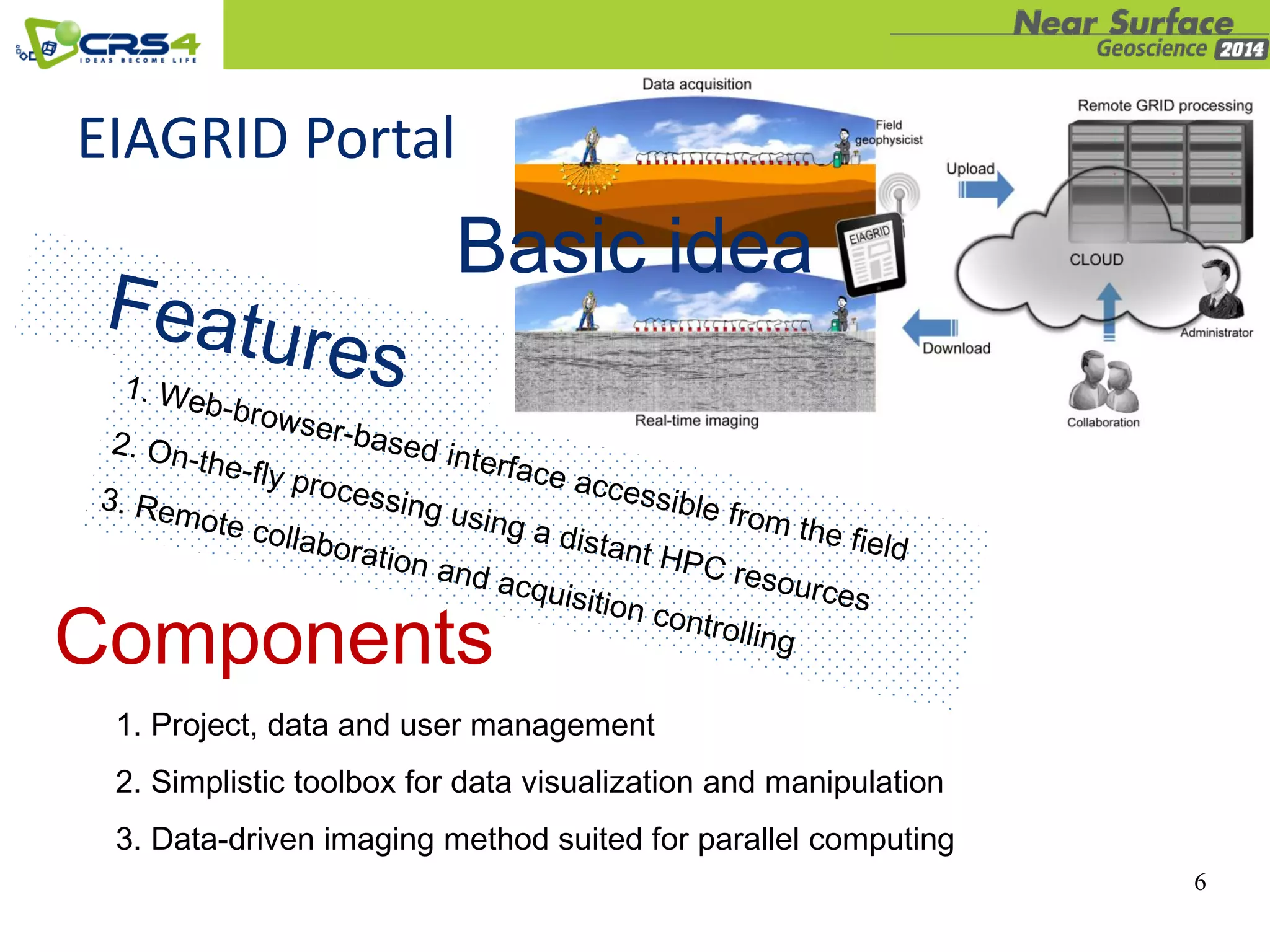
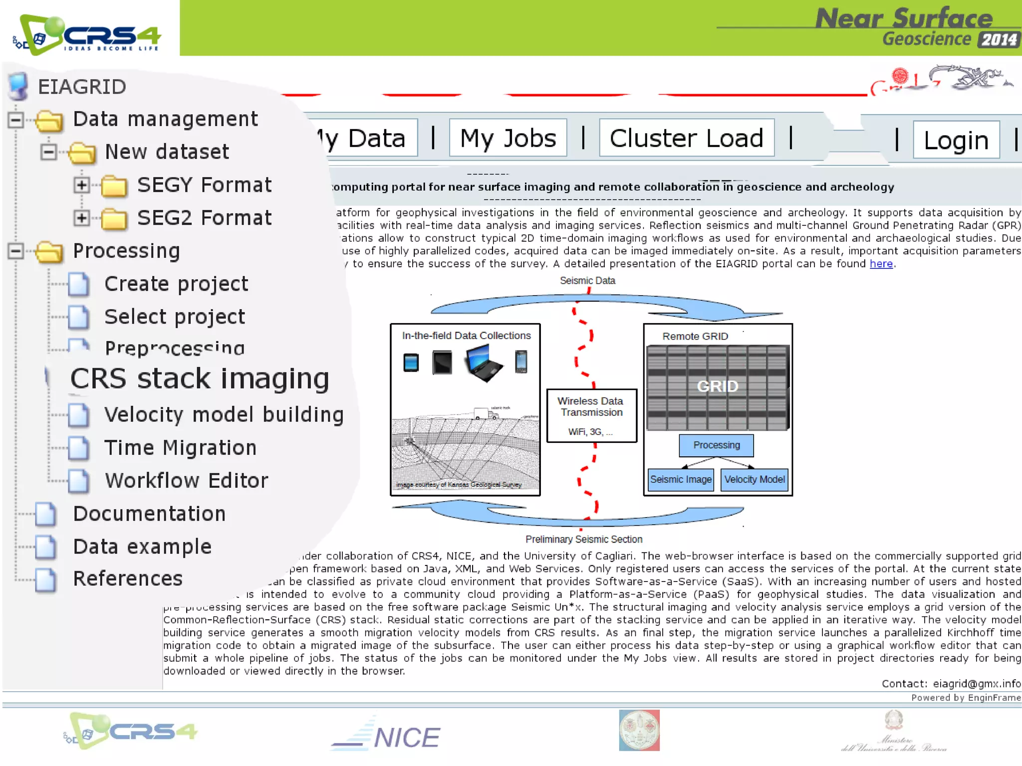
This document describes using a cloud computing portal for real-time and full-precision common reflection surface (CRS) imaging of ground penetrating radar and shallow seismic data. It presents examples of using the portal for real-time multi-offset GPR imaging and full-precision SH-wave imaging. The portal allows 3D parameter searches for high resolution CRS stacking or 3D line searches for rapid real-time imaging directly in the field. Full precision CRS imaging provides higher resolution and more stable velocities than conventional NMO methods for low fold, noisy, or laterally varying data. The cloud computing approach reduces hardware requirements and facilitates the use of data-driven imaging methods for near-surface applications.