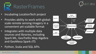
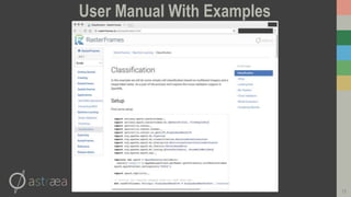
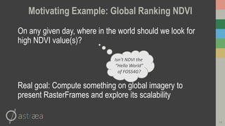
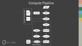
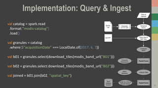
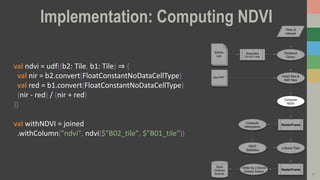
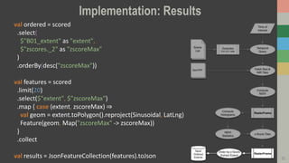
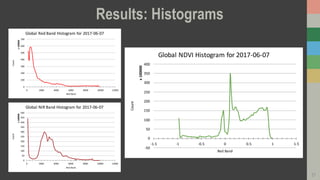
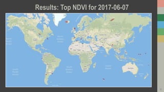
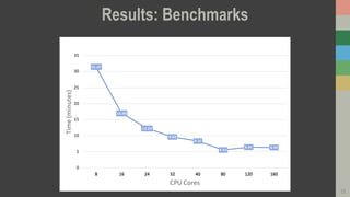
This document introduces RasterFrames, an open source project that enables global-scale geospatial machine learning. RasterFrames provides scalable tools for working with large remote sensing datasets in a convenient format. It integrates with Spark, GeoTrellis and other libraries. The document demonstrates RasterFrames by computing NDVI values from MODIS data and finding the highest NDVI locations globally on a given day. Performance benchmarks show RasterFrames can scale to large datasets across multiple CPU cores.

1. See the Earth as it could be.
Enabling Global-Scale Geospatial Machine Learning
FOSS4G NA 2018
Simeon Fitch
Co-Founder & VP of R&D
Astraea, Inc.

2. See the Earth as it could be. 2
Overview
• Context
• Problem Statement
• Introducing RasterFrames
• Example Problem
• Numerical and Performance Results
• Take-Aways

3. See the Earth as it could be. 3
With exploding population growth and finite resources,
we need to have tools to better plan for sustainable
growth.
By automating the processes around Remote Sensing,
High Performance Computing, and Machine Learning,
we empower individuals to ask complex questions of
the world.
HPC
ML
RS

4. See the Earth as it could be. 4
Think Locally, Compute Globally
• Model development is a creative, iterative, and
interactive process. How do we do this on a global
scale?
• Good tools minimize cognitive friction; attentive to good
ergonomics
• At a minimum, we need:
Solve for local → Scale to global
• Global-scale remote sensing data provide particular
challenges

5. 5
Why This is Hard: Data Dimensionality
Temporal
Spatial
Spectral
Metadata

6. 6
Why This is Hard: Data Density
500 Meter
7 Band
30 Meter
8 Band
3 Meter
4 Band
1 Meter
4 Band
0.3 Meter
8 Band
0
1
10
100
1,000
10,000
100,000
1,000,000
MODIS NBAR Landsat Planet NAIP Digital Globe
MultibandBytes
Football Field Multiband Image in Bytes
Log
Scale!

7. 7
Why This is Hard: Data Velocity
EOSDISHoldingsand Projected Growth
4
Source: Katie Baynes, NASA Goddard. “NASA’s EOSDIS Cumulus”. 2017. https://goo.gl/eQX9om

8. See the Earth as it could be. 8
Why This is Hard: Compute & Mental Model
• Traditional cluster computing (e.g. MPI) scales, but requires
special expertise
• Python Pandas & R DataFrames are very accessible, but not
scalable
• Spark DataFrames provide the best of both worlds, but aren’t
imagery friendly, until now

9. See the Earth as it could be.
• Incubating LocationTech project
• Provides ability to work with global-
scale remote sensing imagery in a
convenient yet scalable format
• Integrates with multiple data
sources and libraries, including
Spark ML, GeoTrellis Map Algebra
and GeoMesa Spark-JTS
• Python, Scala and SQL APIs
GeoTrellis
Layers
Map Algebra
Layer
Operations
Statistical
Analysis
Ti l eLayer RDD Machine
Learning
Visualization
GeoTIFF
RasterFrame
Spark
Dat aSour ce
Spark
Dat aFr ame
spatial
join
Geospatial
Queries
9

10. See the Earth as it could be.
RasterFrame Anatomy
10

11. See the Earth as it could be.
Standard Tile Operations
• localAggStats
• localAggMax
• localAggMin
• localAggMean
• localAggDataCells
• localAggNoDataCells
• localAdd
• localSubtract
• localMultiply
• localDivide
• localAlgebra
• tileDimensions
• aggHistogram
• aggStats
• aggMean
• aggDataCells
• aggNoDataCells
• tileMean
• tileSum
• tileMin
• tileMax
• tileHistogram
• tileStats
• dataCells
• noDataCells
• box2D
• tileToArray
• arrayToTile
• assembleTile
• explodeTiles
• cellType
• convertCellType
• withNoData
• renderAscii
11

12. Polyglot API
12
SELECT spatial_key,
rf_localAggMin(red) as red_min,
rf_localAggMax(red) as red_max,
rf_localAggMean(red) as red_mean
FROM df
GROUP BY spatial_key
df.groupBy("spatial_key").agg(
localAggMin($"red") as "red_min",
localAggMax($"red") as "red_max",
localAggMean($"red") as "red_mean")
df.groupBy(df.spatial_key).agg(
localAggMin(df.red).alias('red_min'),
localAggMax(df.red).alias('red_max'),
localAggMean(df.red).alias('red_mean'))

13. User Manual With Examples
13

14. 14
Motivating Example: Global Ranking NDVI
On any given day, where in the world should we look for
high NDVI value(s)?
Real goal: Compute something on global imagery to
present RasterFrames and explore its scalability
Isn’t NDVI the
“Hello World”
of FOSS4G?

15. Compute Pipeline
15

16. Implementation: Query & Ingest
16
val catalog = spark.read
.format("modis-catalog")
.load()
val granules = catalog
.where($"acquisitionDate" === LocalDate.of(2017, 6, 7))
val b01 = granules.select(download_tiles(modis_band_url("B01")))
val b02 = granules.select(download_tiles(modis_band_url("B02")))
val joined = b01.join(b02, "spatial_key")

17. Implementation: Computing NDVI
17
val ndvi = udf((b2: Tile, b1: Tile) ⇒ {
val nir = b2.convert(FloatConstantNoDataCellType)
val red = b1.convert(FloatConstantNoDataCellType)
(nir - red) / (nir + red)
})
val withNDVI = joined
.withColumn("ndvi", ndvi($"B02_tile", $"B01_tile"))

18. Implementation: Computing Histograms
18
-50
0
50
100
150
200
250
300
350
400
-1.5 -1 -0.5 0 0.5 1 1.5Count
x100000 Red Band
Global NDVI Histogram for 2017-06-07
0
100
200
300
400
500
600
700
0 2000 4000 6000 8000 10000 12000
Count
x100000
Red Band
Global Red Band Histogram for 2017-06-07
0
50
100
150
200
250
300
350
400
450
500
0 2000 4000 6000 8000 10000 12000
Count
x100000
Red Band
Global NIR Band Histogram for 2017-06-07
val hist = withNDVI.select(
aggHistogram($"B01_tile"),
aggHistogram($"B02_tile"),
aggHistogram($"ndvi")
)

19. Implementation: Scoring Tiles
19
val ndviStats = hist.first()._3.stats
val zscoreRange = udf((t: Tile) ⇒ {
val mean = ndviStats.mean
val stddev = math.sqrt(ndviStats.variance)
t.mapDouble(c ⇒ (c - mean) / stddev).findMinMaxDouble
})
val scored = withNDVI
.withColumn("zscores", zscoreRange($"ndvi"))

20. Implementation: Results
20
val ordered = scored
.select(
$"B01_extent" as "extent",
$"zscores._2" as "zscoreMax"
)
.orderBy(desc("zscoreMax"))
val features = scored
.limit(20)
.select($"extent", $"zscoreMax")
.map { case (extent, zscoreMax) ⇒
val geom = extent.toPolygon().reproject(Sinusoidal, LatLng)
Feature(geom, Map("zscoreMax" -> zscoreMax))
}
.collect
val results = JsonFeatureCollection(features).toJson

21. Results: Histograms
0
100
200
300
400
500
600
700
0 2000 4000 6000 8000 10000 12000
Count
x100000
Red Band
Global Red Band Histogram for 2017-06-07
-50
0
50
100
150
200
250
300
350
400
-1.5 -1 -0.5 0 0.5 1 1.5
Count
x100000
Red Band
Global NDVI Histogram for 2017-06-07
0
50
100
150
200
250
300
350
400
450
500
0 2000 4000 6000 8000 10000 12000
Count
x100000
Red Band
Global NIR Band Histogram for 2017-06-07
21

22. Results: Top NDVI for 2017-06-07
22

23. Results: Benchmarks
23
31.47
16.99
12.23
9.64
8.31
5.53
6.41 6.33
0
5
10
15
20
25
30
35
8 16 24 32 40 80 120 160
Time(minutes)
CPU Cores

24. See the Earth as it could be. 24
RasterFrame Take-Aways
• DataFrames lower cognitive friction when modeling. Good
Ergonomics!
• Rich set of raster processing primitives
• Support for descriptive and predictive analysis
• Via spark-shell, Jupyter Notebook, Zeppelin, etc. can
interact with data and iterate over solution
• It scales!
• Many more examples at http://rasterframes.io

25. See the Earth as it could be. 25
Getting Started
• Try it out via Jupyter Notebooks:
docker pull s22s/rasterframes-notebooks
• Documentation: http://rasterframes.io
• Code: https://github.com/locationtech/rasterframes
• Chat: https://gitter.im/s22s/raster-frames
• Social: @metasim on GitHub & Twitter
• Company: http://www.astraea.earth

26. See the Earth as it could be. 26
Shout Outs
• Thanks to LocationTech
• For Incubating RasterFrames; mentoring by Jim Hughes & Rob Emanuele
• The teams behind GeoTrellis, GeoMesa, JTS, & SFCurve
• Thanks to NASA, USGS, & NOAA
• Supporting public access to massive curated data sets is not easy!
• Upcoming Astraea Presentations
• Machine Learning, FOSS, and open data to map deforestation trends in the Brazilian Amazon
Courtney Whalen & Jason Brown
Tuesday, May 15, 2018 - 4:30 to 5:05 (right after this presentation)
Gateway 1
• Using Deep Learning to Derive 3D Cities from Satellite Imagery
Eric Culbertson
Wednesday, May 16, 2018 - 2:00 to 2:35
Gateway 2
• Please visit Astraea
• Booth #14