Random Numbers andVariates
Introduction to Random Number Generation
Important Considerations for Random Number
Generation
Techniques for Generating Random
Numbers
Linear Congruential Method
Combined Linear Congruential Generators
Chi-SquareTest
Acceptance-RejectionTechnique
3.
Random Number Generation
Random numbers are a necessary basic ingredient
in the simulation of almost all discrete systems.
Most computer languages have a subroutine, object,
or function that will generate a random number.
Similarly, simulation languages generate random
numbers that are used to generate event times and
other random variables.
4.
Important Considerations forRandom
Number Generation
(1) The routine should be fast.
Individual computations are inexpensive, but simulation could
require many millions of random numbers.
The total cost can be managed by selecting a computationally
efficient method of random number generation.
(2) The routine of generating random numbers
should be portable to different computers and
programming languages.
This is desirable so that the simulation program will produce
the same results wherever it is executed.
5.
Important Considerations
(3)The routine of generating random numbers
should have a sufficiently long cycle.
The cycle length, or period, represents the length of the
random number sequence before previous numbers begin to
repeat themselves in an earlier order.
(4) The random numbers should be replicable.
Given the starting point (or conditions) it should be possible
to generate the same set of random numbers completely
independent of the system that is being simulated.
This is helpful for debugging purposes and is a means of
facilitating comparisons between systems.
6.
Important Considerations
(5)Most important, the generated random numbers
should closely approximate the ideal statistical properties
of uniformity and independence.
(See Properties of Random Numbers)
Techniques for GeneratingRandom
Numbers
Linear Congruential Method (LCM).
Combined Linear Congruential Generators (CLCM).
9.
(1) Linear CongruentialMethod
The linear congruential method, initially proposed by
Lehmer [1951], produces a sequence of integers, x1, x2, ...
between zero and (m – l) by following a recursive
relationship:
(X0) is the initial value, it is called the seed
(a) is called the multiplier
(c) is the increment
(m) is the modulus
If c ≠ 0, then the form is called the mixed congruential
method, when c = 0, the form is known as the
multiplicative congruential method.
Xi+1 = (aXi + c) mod m where i = 0, I, 2, ...
10.
(1) Linear CongruentialMethod
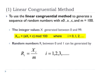
To use the linear congruential method to generate a
sequence of random numbers with x0 , a , c, and m = 100.
The integer values X generated between 0 and 99.
Random numbers Ri between 0 and 1 can be generated by
,......
3
,
2
,
1
i
m
X
R i
i
Xi+1 = (aXi + c) mod 100 where i = 0, I, 2, ...
11.
Note
The seedfor a linear congruential random-number
generator:
Is the integer value X0 that initializes the random-number
sequence.
Any value in the sequence can be used to “seed” the generator.
12.
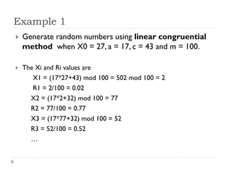
Example 1
Generaterandom numbers using linear congruential
method when X0 = 27, a = 17, c = 43 and m = 100.
The Xi and Ri values are
X1 = (17*27+43) mod 100 = 502 mod 100 = 2
R1 = 2/100 = 0.02
X2 = (17*2+32) mod 100 = 77
R2 = 77/100 = 0.77
X3 = (17*77+32) mod 100 = 52
R3 = 52/100 = 0.52
…
13.
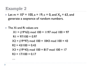
Example 2
Letm = 102 = 100, a = 19, c = 0, and X0 = 63, and
generate a seqnence of random numbers.
The Xi and Ri values are
X1 = (19*63) mod 100 = 1197 mod 100 = 97
R1 = 97/100 = 0.97
X2 = (19*97) mod 100 = 1843 mod 100 = 43
R2 = 43/100 = 0.43
X3 = (19*43) mod 100 = 817 mod 100 = 17
R3 = 17/100 = 0.17
…
14.
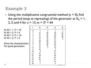
Example 3
Usingthe multiplicative congruential method (c = 0), find
the period (stop at repreating) of the generator at X0 = 1,
2, 3, and 4 for a = 13, m = 26 = 64
At X0 = 1, P = 16
At X0 = 2, P = 8
At X0 = 3, P = 16
At X0 = 4, P = 4
Show the characteristics
For good generators
15.
Characteristics of aGood Generator
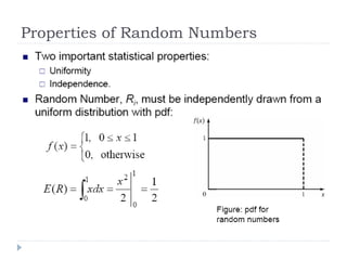
Maximum Density
Such that the values assumed by Ri, i = 1,2,…, leave no large
gaps on [0,1]
Problem: Instead of continuous, each Ri is discrete
Solution: a very large integer for modulus m
Approximation appears to be of little consequence
Maximum Period
To achieve maximum density and avoid cycling.
Achieve by: proper choice of a, c, m, and X0.
Most digital computers use a binary representation of
numbers
Speed and efficiency are aided by a modulus, m, to be (or close
to) a power of 2.
16.
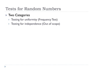
Tests for RandomNumbers
Two Categories
Testing for uniformity (FrequencyTest)
Testing for independence (Out of scope)
17.
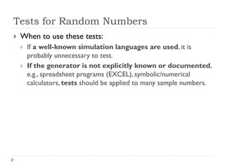
Tests for RandomNumbers
When to use these tests:
If a well-known simulation languages are used, it is
probably unnecessary to test.
If the generator is not explicitly known or documented,
e.g., spreadsheet programs (EXCEL), symbolic/numerical
calculators, tests should be applied to many sample numbers.
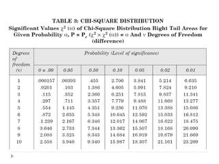
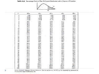
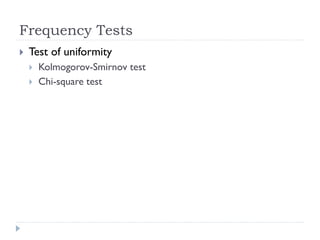
(2) Chi-square Test
Chi-square test measures the degree of agreement
between the distribution of a sample of generated
random numbers and the theoretical uniform
distribution.
The chi-square is valid only for large samples, say N >= 50
(no. of classes 5-10)
Oi is the observed number in the ith class.
Ei is the expected number in the ith class
n is the number of classes.
For the uniform distribution, Ei, the expected number in
each class is given by Ei = N/n (Null hypothesis: H0)
n
i i
i
i
E
E
O
1
2
2
0
20.
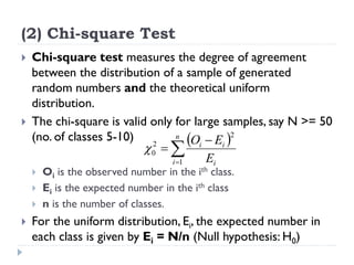
Example
Use thechi-square test at 0.05 to test for whether the data
shown next are uniformly distributed.
O1 =(0, 0.1] = {0.06, 0.01, 0.05, 0.05, 0.1, 0.02, 0.05, 0.05} = 8
E1 = {0.01, 0.02, 0.03, 0.04, 0.05, 0.06, 0.07, 0.08, 0.09, 0.1} = 10
21.
Example
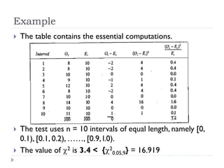
The tablecontains the essential computations.
The test uses n = 10 intervals of equal length, namely [0,
0.1), [0.1, 0.2), ……, [0.9, l.0).
The value of 2 is 3.4 < {2
0.05,9} = 16.919

![(1) Linear Congruential Method
The linear congruential method, initially proposed by
Lehmer [1951], produces a sequence of integers, x1, x2, ...
between zero and (m – l) by following a recursive
relationship:
(X0) is the initial value, it is called the seed
(a) is called the multiplier
(c) is the increment
(m) is the modulus
If c ≠ 0, then the form is called the mixed congruential
method, when c = 0, the form is known as the
multiplicative congruential method.
Xi+1 = (aXi + c) mod m where i = 0, I, 2, ...](https://image.slidesharecdn.com/lec6-250930070406-42521d99/85/Lec6-computer-simulation-Modeling-and-Simulation-pdf-9-320.jpg)
![Characteristics of a Good Generator
Maximum Density
Such that the values assumed by Ri, i = 1,2,…, leave no large
gaps on [0,1]
Problem: Instead of continuous, each Ri is discrete
Solution: a very large integer for modulus m
Approximation appears to be of little consequence
Maximum Period
To achieve maximum density and avoid cycling.
Achieve by: proper choice of a, c, m, and X0.
Most digital computers use a binary representation of
numbers
Speed and efficiency are aided by a modulus, m, to be (or close
to) a power of 2.](https://image.slidesharecdn.com/lec6-250930070406-42521d99/85/Lec6-computer-simulation-Modeling-and-Simulation-pdf-15-320.jpg)
![Example
Use the chi-square test at 0.05 to test for whether the data
shown next are uniformly distributed.
O1 =(0, 0.1] = {0.06, 0.01, 0.05, 0.05, 0.1, 0.02, 0.05, 0.05} = 8
E1 = {0.01, 0.02, 0.03, 0.04, 0.05, 0.06, 0.07, 0.08, 0.09, 0.1} = 10](https://image.slidesharecdn.com/lec6-250930070406-42521d99/85/Lec6-computer-simulation-Modeling-and-Simulation-pdf-20-320.jpg)