Download as PDF, PPTX

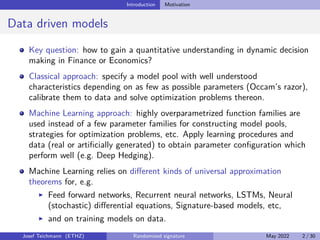
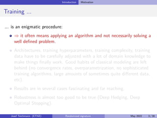
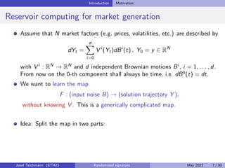

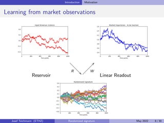
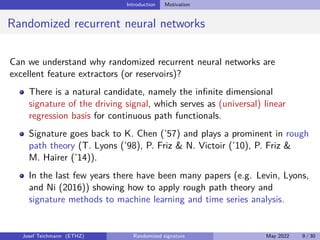


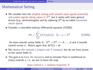
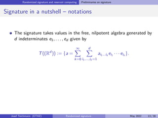
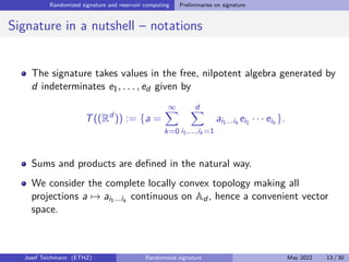
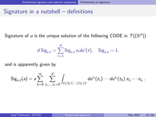
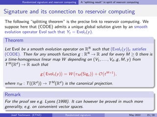

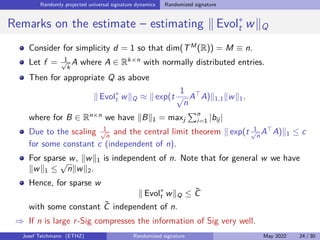
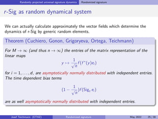
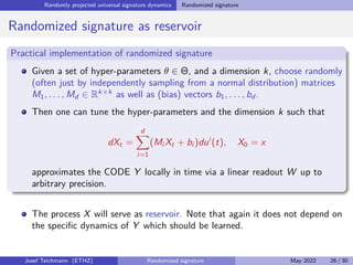
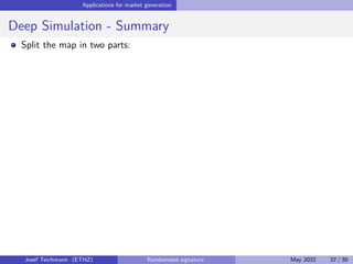
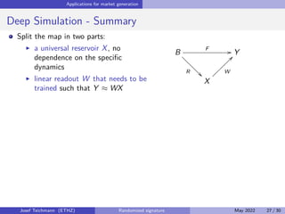
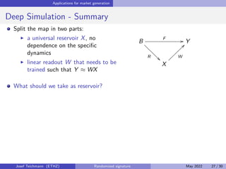
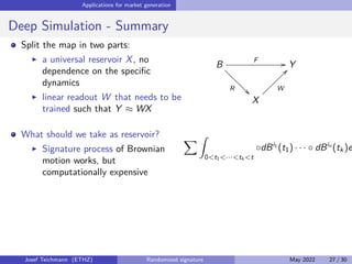
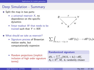

The document discusses using randomized recurrent neural networks and signature-based methods for machine learning in finance. It proposes splitting the input-output map of a dynamical system into a "reservoir" part and a linear "readout" part. The signature of the input signal provides a natural candidate for the reservoir, as it is point-separating and linear functions on the signature can approximate continuous functionals via the universal approximation theorem. The goal of the talk is to prove how dynamical systems can be approximated using randomized recurrent networks, with precise convergence rates, and to view randomized deep networks through this lens.