Download as PDF, PPTX


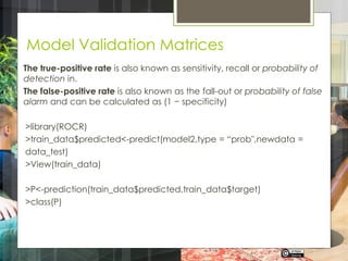
![Interpreting ROCR curve
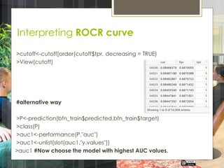
#Tpr and Fpr are the arguments of the “performance” function
indicating that the plot is between true positive & false positive rate.
>pref<-performance (P, "tpr", "fpr")
>class(pref)
#now this will give confusion matrix for all possible cut off values
>plot(pref,col=“red”)
#plot the absolute line
>abline(0,1, lty=8, col=“grey”)
Basically TPR should be greater than FPR
than the model is considered to be good
#now convert it into a data frame
>cutoff<-
data.frame(cut=pref@alpha.values[[1]],fpr=pref@x.values[[1]],tpr=pref
@y.values[[1]] )
Rupak Roy](https://image.slidesharecdn.com/10-220113051853/85/Random-Forest-Bootstrap-Aggregation-13-320.jpg)


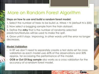
Random Forest is a powerful machine learning algorithm that utilizes ensemble methods like bagging to improve predictive accuracy by averaging multiple decision trees built from random samples of features. It reduces variance without increasing bias, allows for the use of out-of-bag samples for model validation, and handles missing values and outliers effectively. Compared to boosting and other algorithms, Random Forest is faster in processing large datasets and requires less data pre-processing.