Download as PDF, PPTX
![Network analysis
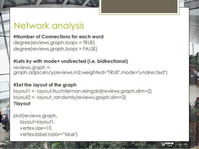
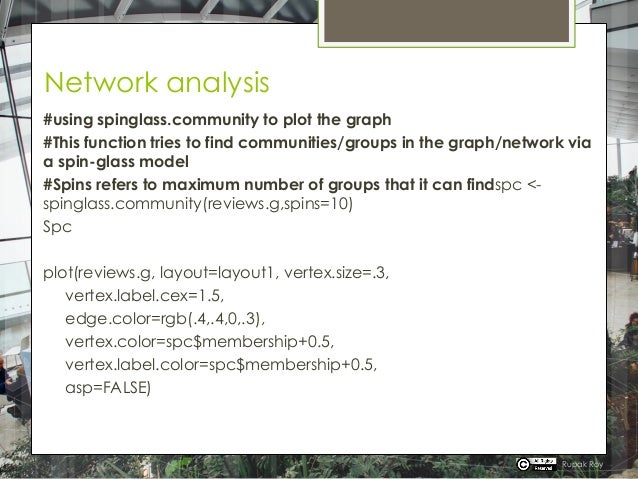
#Network analysis now will help us to understand how many
connections a specific word has with other words.
#The keywords will be the “node”s in the network, and the
#Connections are will be called as edges
#read the data
reviews<-read.csv(file.choose(),stringsAsFactors=FALSE,nrows = 500)
View(reviews)
names(reviews)
reviews1<-data.frame(reviews$reviews.text)
names(reviews1)
dim(reviews1)
names(reviews1)[1]<-"reviews"
Rupak Roy](https://image.slidesharecdn.com/5-220114111304/95/Network-Analysis-NLP-4-638.jpg)
![Network analysis
#Build a Text Corpus
library(tm)
review.corpus<-Corpus(VectorSource(reviews1$reviews))
summary(review.corpus)
inspect(review.corpus[1:5]) #Inspecting elements in Corpus
#Data Transformations -Cleaning
#Converting to lower case
review.corpus<-tm_map(review.corpus,tolower)
#Removing extra white space
review.corpus<-tm_map(review.corpus,stripWhitespace)
#Removing punctuations
review.corpus<-tm_map(review.corpus,removePunctuation)
#Removing numbers
review.corpus<-tm_map(review.corpus,removeNumbers)
#Can add more words apart from standard list
my_stopwords<-c(stopwords('english'),'@','http*','url','www*')
review.corpus<-tm_map(review.corpus,removeWords,my_stopwords)
Rupak Roy](https://image.slidesharecdn.com/5-220114111304/95/Network-Analysis-NLP-5-638.jpg)
![Network analysis
library(igraph)
# Convert to tdm
reviews.tdm <-
TermDocumentMatrix(tweets.corpus,control=list(wordLengths=c(1, Inf)))
#Remove sparse terms
reviews.tdm.rm <- removeSparseTerms(reviews.tdm, sparse=0.95)
inspect(obama.tdm.rm[1:10,1:10])
#Transform the tdm to a matrix format.
reviews.m <- as.matrix(reviews.tdm.rm)
#convert the matrix values to 2 level factor 1/0(i.e. 'Yes' or 'No')
indicating 1 for existng values other than zero
reviews.m[reviews.m>=1] <- 1
Rupak Roy](https://image.slidesharecdn.com/5-220114111304/95/Network-Analysis-NLP-6-638.jpg)
![Network analysis
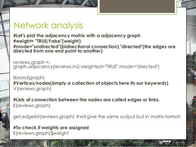
#Build Term Adjacency matrix which will show us how many
connections each TERM has.
#This is done by using the product of 2 matrices and the output will be
the number of times each term appears together in a document
reviews.m2 <- reviews.m %*% t(reviews.m)
reviews.m2[1:10,1:10]
#We can see the times each term/word occurred with other words.
Rupak Roy](https://image.slidesharecdn.com/5-220114111304/95/Network-Analysis-NLP-7-638.jpg)

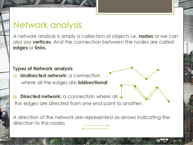
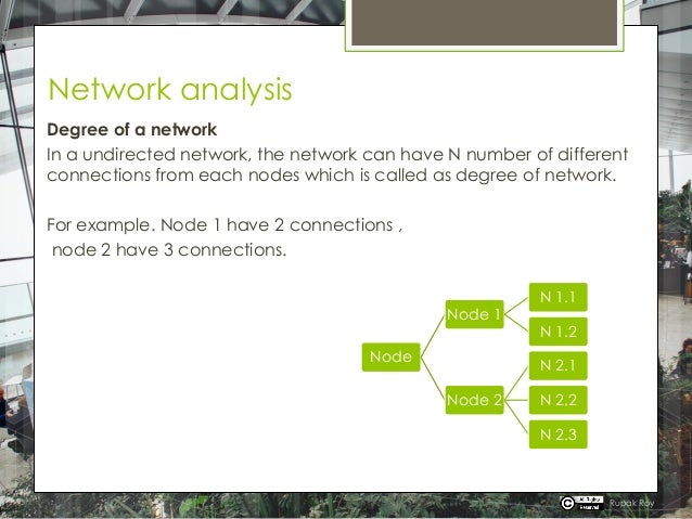
The document discusses network analysis, defining key concepts such as nodes and edges, and differentiating between directed and undirected networks. It outlines the process of analyzing text data, including cleaning, creating a term-document matrix, and plotting 3D and interactive visualizations of the network. Various techniques for visualizing and analyzing the connections between terms in the data are also presented.