
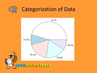
![Categorization of Data> salary <- c(23,2,34,1,32,22,45,3,4,5,12)> bins <- cut(salary, breaks=c(0,10,20,30,40,max(salary)))> bins [1] (20,30] (0,10] (30,40] (0,10] (30,40] (20,30] [7] (40,45] (0,10] (0,10] (0,10] (10,20]Levels: (0,10] (10,20] (20,30] (30,40] (40,45]> table(bins)bins (0,10] (10,20] (20,30] (30,40] (40,45] 5 1 2 2 1 > pie(table(bins))](https://image.slidesharecdn.com/3-9rstatistics-100122124153-phpapp01/85/R-Statistics-13-320.jpg)
![Histograms> data [1] 2 3 1 3 2 4 1 2 4 1 3 4 1 2 1 2 3 2 5 4 1[22] 2 3 4 3 2 4 3> hist(data)> rug(jitter(data))](https://image.slidesharecdn.com/3-9rstatistics-100122124153-phpapp01/85/R-Statistics-15-320.jpg)

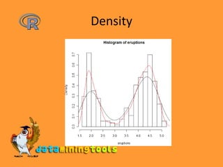

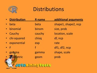
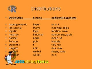
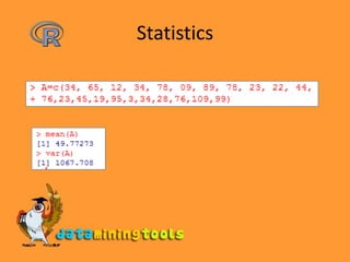
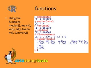
This document provides an overview of statistical functions and graphs available in R. It lists common distributions that can be evaluated or simulated in R, including beta, binomial, Cauchy, chi-squared, exponential, F, gamma, geometric, hypergeometric, log-normal, logistic, negative binomial, normal, Poisson, Student's t, uniform, and Weibull. It also discusses functions for calculating median, mean, variance, standard deviation, five number summary, and generating stem-and-leaf plots, histograms, density plots, bar plots, pie charts in R. Categorical data can be grouped using the cut function and summarized using table.