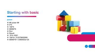
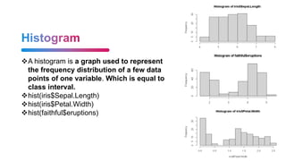
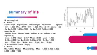
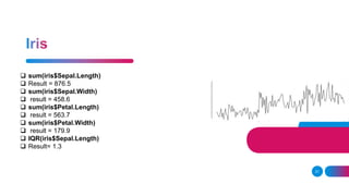
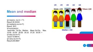
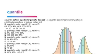
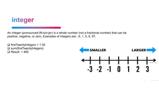
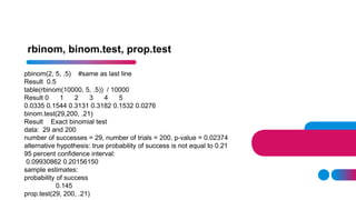
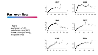
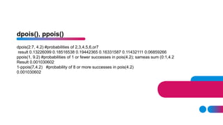
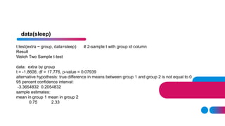
The document provides a comprehensive guide on using R programming, covering basic calculations such as addition, subtraction, multiplication, and division. It also introduces key concepts like data frames, pie charts, histograms, and statistical functions including summary statistics, quantiles, and regression analysis. Additionally, it includes practical examples for creating plots and performing sampling and probability distributions.


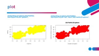
![Repetition and sequence
10
##rep()##
rep(3,10)
Result = 3 3 3 3 3 3 3 3 3 3
• rep(90,9)
result = 90 90 90 90 90 90 90 90 90
##seq()
• Seq (1,100)
= Result
[1] 1 2 3 4 5 6 7 8 9 10 11 12 13 14 15 16 17 18 19
[20] 20 21 22 23 24 25 26 27 28 29 30 31 32 33 34 35 36 37 38
[39] 39 40 41 42 43 44 45 46 47 48 49 50 51 52 53 54 55 56 57
[58] 58 59 60 61 62 63 64 65 66 67 68 69 70 71 72 73 74 75 76
[77] 77 78 79 80 81 82 83 84 85 86 87 88 89 90 91 92 93 94 95
[96] 96 97 98 99 100](https://image.slidesharecdn.com/rstudiopresentation-231124170750-b341f72b/85/r-studio-presentation-pptx-10-320.jpg)
![Letters, LETTER, month.abb, month.name
12
Letters
"a" "b" "c" "d" "e" "f" "g" "h" "i" "j" "k" "l" "m" "n" "o" "p" "q" "r" "s" "t"
"u" "v" "w" "x" "y" "z"
LETTERS
"A" "B" "C" "D" "E" "F" "G" "H" "I" "J" "K" "L" "M" "N" "O" "P" "Q" "R"
"S" "T" [21] "U" "V" "W" "X" "Y" "Z"
month.abb
"Jan" "Feb" "Mar" "Apr" "May" "Jun" "Jul" "Aug" "Sep" "Oct" "Nov"
"Dec“
month.name
"January" "February" "March" "April" "May" "June"
[7] "July" "August" "September" "October" "November"
"December"](https://image.slidesharecdn.com/rstudiopresentation-231124170750-b341f72b/85/r-studio-presentation-pptx-12-320.jpg)
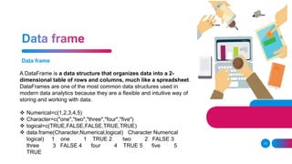
![It is basically a table where each column is a variable and each row has one
set of values for each of those variables (much like a single sheet in a program
like LibreOffice Calc or Microsoft Excel).
18
Basic
data("iris")
names(iris)
Result "Sepal.Length" "Sepal.Width" "Petal.Length" "Petal.Width" "Species"
dim(iris)
Result = 150 5
str(iris3)
num [1:50, 1:4, 1:3] 5.1 4.9 4.7 4.6 5 5.4 4.6 5 4.4 4.9 ...
- attr(*, "dimnames")=List of 3
..$ : NULL
..$ : chr [1:4] "Sepal L." "Sepal W." "Petal L." "Petal W."
..$ : chr [1:3] "Setosa" "Versicolor" "Virginica"](https://image.slidesharecdn.com/rstudiopresentation-231124170750-b341f72b/85/r-studio-presentation-pptx-18-320.jpg)
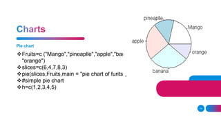
![replicate
sample(c("heads","TAILS"), 2, replace = T)
Result "TAILS" "heads"
replicate(5, sample(c("Heads","TAILS"), 2, replace =T))
Result [,1] [,2] [,3] [,4] [,5]
[1,] "Heads" "Heads" "Heads" "Heads" "Heads"
[2,] "Heads" "Heads" "Heads" "Heads" "Heads"
replicate(10, sample(c("Heads","TAILS"), 2, replace =T))
Result](https://image.slidesharecdn.com/rstudiopresentation-231124170750-b341f72b/85/r-studio-presentation-pptx-35-320.jpg)
![data(warpbreaks)
by(warpbreaks$breaks, warpbreaks$tension, mean)
warpbreaks$tension: L
[1] 36.38889
---------------------------------------------------------------
warpbreaks$tension: M
[1] 26.38889
---------------------------------------------------------------
warpbreaks$tension: H
[1] 21.66667
by](https://image.slidesharecdn.com/rstudiopresentation-231124170750-b341f72b/85/r-studio-presentation-pptx-40-320.jpg)
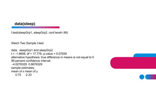


![[1062BPY12001] Data analysis with R / week 2](https://cdn.slidesharecdn.com/ss_thumbnails/dataanalyzer01-180307063046-thumbnail.jpg?width=640&height=640&fit=bounds)


