BIO360 Biometrics I, Fall 2007
1
R cheat sheet
1. Basics
Commands objects() List of objects in workspace
ls() Same
rm(object) Delete ‘object’
Assignments <- Assign value to a variable
= Same
Getting help help(fun) Display help file for function fun()
args(fun) List arguments of function fun()
Libraries / packages library(pkg) Open package (library) ‘pkg’
library(help=pkg) Display description of package ‘pkg’
2. Vectors and data types
Generating seq(-4,4,0.1) Sequence: -4.0, -3.9, -3.8, ..., 3.9, 4.0
2:7 Same as seq(2,7,1)
c(5,7,9,1:3) Concatenation (vector): 5 7 9 1 2 3
rep(1,5) 1 1 1 1 1
rep(4:6,1:3) 4 5 5 6 6 6
gl(3,2,12) Factor with 3 levels, repeat each level in blocks
of 2, up to length 12 (1 1 2 2 3 3 1 1 2 2 3 3)
Coercion as.numeric(x) Convert to numeric
as.character(x) Convert to text string
as.logical(x) Convert to logical
factor(x) Create factor from vector x
unlist(x) Convert list, result from table() etc. to vector
3. Data frames
Accessing data data.frame(height,
weight)
Collect vectors ‘height’ and ‘weight’ into
data frame
dfr&var Select vector ‘var’ in data frame ‘dfr’
attach(dfr) Put data frame in search path
detach() - and remove it from the path
Editing dfr2 <- edit(dfr) open data frame ‘dfr’ in spreadsheet, write
changed version into new data frame ‘dfr2’
fix(dfr) open data frame ‘dfr’ in spreadsheet,
changes will overwrite entries in ‘dfr’
Summary dim(dfr) Number of rows and columns in data frame
‘dfr’, works also for matrices and arrays
summary(dfr) Summary statistics for each variable in ‘dfr’
H. Wagner, Biology UTM
2
Modified from: P. Dalgaard (2002). Introductory Statistics with R. Springer, New York.
4. Input and export of data
General data(name) Built-in data set
read.table(“file.txt”) Read from external ASCII file
Arguments to
read.table()
header = TRUE First line has variable names
row.names = 1 First column has row names
sep = “,” Data are separated by commas
sep = “t” Data are separated by tabs
dec = “,” Decimal point is comma
na.strings = “.” Missing value is dot
Variants of
read.table()
read.csv(“file.csv”) Comma separated
read.delim(“file.txt”) Tab delimited text file
Export write.table() see help(write.table) for details
Adding names names() Column names for data frame or list only
dimnames() Row and column names, also for matrix
5. Indexing / selection / sorting
Vectors x[1] First element
x[1:5] Subvector containing the first five elements
x[c(2,3,5)] Elements nos. 2, 3, and 5
x[y <= 30] Selection by logical expression
x[sex = = “male”] Selection by factor variable
i <-c(2,3,5); x[i] Selection by numerical variable
k <- (y <=30); x[k] Selection by logical variable
length(x) Returns length of vector x
Matrices, data
frames
m[4, ] Fourth row
m[ ,3] Third column
drf[drf$var <=30, ] Partial data frame (not for matrices)
subset(dfr,var<=30) Same, often simpler (not for matrices)
m[m[ ,3]<=30, ] Partial matrix (also for data frames)
Sorting sort(c(7,9,10,6)) Returns the sorted values: 6, 7, 9, 10
order(c(7,9,10,6)) Returns the element number in order of
ascending values: 4, 1, 2, 3
order(c(7,9,10,6),
decreasing = TRUE)
same, but in order of decreasing values:
3, 2, 1, 4
rank(c(7,9,10,6)) Returns the ranks in order of ascending
values: 2, 3, 4, 1
BIO360 Biometrics I, Fall 2007
3
6. Missing values
Functions is.na(x) Logical vector. TRUE where x has NA
complete.cases(x1,x2,...) Neither missing in x1, nor x2, nor ...
Arguments to
other functions
na.rm = In statistical functions: Remove
missing if TRUE, returns NA if FALSE
na.last = In ‘sort’ TRUE, FALSE and NA means
“last”, “first”, and “discard”
na.action = in ‘lm()’, etc., values na.fail,
na.omit, na.exclude
na.print = In ‘summary()’ and ‘print()’:
How to represent NA in output
na.strings = In ‘read.table()’:
Codes(s) for NA in input
7. Numerical functions
Mathematical log(x) Logarithm of x, natural logarithm
log(x, 10) Base10 logarithm of x
exp(x) Exponential function ex
sin(x) Sine
cos(x) Cosine
tan(x) Tangent
asin(x) Arcsin (inverse sine)
min(x) Smallest value in vector
min(x1, x2, ...) minimum number over several vectors
max(x) Largest value in vector
range(x) Like c(min(x), max(x))
pmin(x1, x2, ...) Parallel (elementwise) minimum over
multiple equally long vectors
length(x) Number of elements in vector
sum(x) Sum of values in vector
cumsum(x) Cumulative sum of values in vector
sum(complete.cases(x)) Number of non-missing elements
Statistical mean(x) Average
median(x) Median
quantile(x, p) Quantiles: median = quantile(x, 0.5)
var(x) Variance
sd(x) Standard deviation
cor(x, y) Pearson correlation
cor(x, y, method =
“spearman”)
Spearman rank correlation
H. Wagner, Biology UTM
4
8. Programming
Conditional
execution
if(p< 0.5)
print(“Hooray”)
Print “Hooray” if condition is true
if(p < 0.5)
{ print(“Hooray”)
i = i + 1 }
If condition is true, perform all commands
within the curved brackets { }
if(p < 0.5)
{ print(“Hooray”)}
else
{ i = i + 1}
Conditional execution with an alternative
Loop for(i in 1:10)
{ print(i) }
Go through loop 10 times
i <- 1
while(i <= 10)
{ print(i)
i = i + 1 }
Same, but more complicated
User-defined
function
fun<- function(a, b,
doit = FALSE)
{ if(doit) {a + b}
else 0 }
Defines a function ‘fun’ that returns the
sum of a and b if the argument ‘doit’ is
set to TRUE, or zero, if ‘doit’ is FALSE
9. Operators
Arithmetic + Addition
- Subtraction
* Multiplication
/ Division
^ Raise to the power of
% / % Integer division: 5 %/% 3 = 1
% % Remainder from integer division: 5 %% 3 = 2
Logical or relational = = Equal to
! = Not equal to
< Less than
> Greater than
< = Less than or equal to
> = Greater than or equal to
is.na(x) Missing?
& Logical AND
| Logical OR
! Logical NOT
BIO360 Biometrics I, Fall 2007
5
10. Tabulation, grouping, recoding
General table(x) Frequency table of vector (factor) x
table(x, y) Crosstabulation of x and y
xtabs(~ x + y) Formula interface for crosstabulation:
use summary() for chi-square test
factor(x) Convert vector to factor
cut(x, breaks) Groups from cutpoints for continuous
variable, breaks is a vector of cutpoints
Arguments to
factor()
levels = c() Values of x to code. Use if some values
are not present in data, or if the order
would be wrong.
labels = c() Values associated with factor levels
exclude = c() Values to exclude. Default NA. Set to NULL
to have missing values included as a level.
Arguments to
cut()
breaks = c() Cutpoints. Note values of x outside of
‘breaks’ gives NA. Can also be a single
number, the number of cutpoints.
labels = c() Names for groups. Default is 1, 2, ...
Factor recoding levels(f) <- names New level names
factor(newcodes[f]) Combining levels: ‘newcodes’, e.g.,
c(1,1,1,2,3) to amalgamate the first 3
of 5 groups of factor f
11. Manipulations of matrices and lists
Matrix algebra m1 % * % m2 Matrix product
t(m) Matrix transpose
m[lower.tri(m)] Returns the values from the lower triangle
of matrix m as a vector
diag(m) Returns the diagonal elements of matrix m
matrix(x, dim1, dim2) Fill the values of vector x into a new
matrix with dim1 rows and dim2 columns,
Marginal
operations etc.
apply(m, dim, fun) Applies the function ‘fun’ to each row
(dim = 1) or column (dim= 2) of matrix m
tapply(m, list(f1,
f2), fun)
Can be used to aggregate columns or rows
within matrix m as defined by f1, f2, using
the function ‘fun’ (e.g., mean, max)
split(x, f) Split vector, matrix or data frame by
factor x. Different results for matrix and
data frame! The result is a list with one
object for each level of f.
sapply(list, fun)
sapply(split(x,f),
fun)
applies the function ‘fun’ to each object in
a list, e.g. as created by the split function
H. Wagner, Biology UTM
6
12. Statistical standard methods
Parametric tests,
continuous data
t.test One- and two-sample t-test
pairwise.t.test Pairwise comparison of means
cor.test Significance test for correlation coeff.
var.test Comparison of two variances (F-test)
lm(y ~ x) Regression analysis
lm(y ~ f) One-way analysis of variance
lm(y ~ x1 + x2 + x3) Multiple regression
lm(y ~ f1 * f2) Two-way analysis of variance
Non-parametric wilcox.test One- and two-sample Wilcox test
kruskal.test Kruskal-Wallis test
friedman.test Friedman’s two-way analysis of variance
cor.test variant method = “spearman” Spearman rank correlation
Discrete response binom.test Binomial test (incl. sign test)
prop.test Comparison of proportions
fisher.test Exact test in 2 x 2 tables
chisq.test Chi-square test of independence
glm(y ~ x1+x2,
binomial)
Logistic regression
13. Statistical distributions
Normal
distribution
dnorm(x) Density function
pnorm(x) Cumulative distribution function P(X<=x)
qnorm(p) p-quantile, returns x in: P(X<=x) = p
rnorm(n) n random normally distributed numbers
Distributions pnorm(x, mean, sd) Normal
plnorm*x, mean, sd) Lognormal
pt(x, df) Student’s t distribution
pf(x, n1, n2) F distribution
pchisq(x, df) Chi-square distribution
pbinom(x, n, p) Binomial
ppois(x, lambda) Poisson
punif(x, min, max) Uniform
pexp(x, rate) Exponential
pgamma(x, shape,
scale)
Gamma
pbeta(x, a, b) Beta
BIO360 Biometrics I, Fall 2007
7
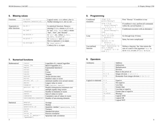
14. Models
Model formulas ~ As explained by
+ Additive effects
: Interaction
* Main effects + interaction: a*b
=a+b+a:b
-1 Remove intercept
Linear models lm.out <- lm(y ~ x) Fit model and save results as ‘lm.out’
summary(lm.out) Coefficients etc.
anova(lm.out) Analysis of variance table
fitted(lm.out) Fitted values
resid(lm.out) Residuals
predict(lm.out,newdata) Predictions for a new data frame
Other models glm(y ~ x, binomial) Logistic regression
glm(y ~ x, poisson) Poisson regression
gam(y ~ s(x)) General additive model for non-linear
regression with smoothing. Package:
gam
tree(y ~ x1+x2+x3) Classification (y = factor) or regression
(y = numeric) tree. Package: tree
Diagnostics rstudent(lm.out) Studentized residuals
dfbetas(lm.out) Change in standardized regression
coefficients beta if observation removed
dffits(lm.out) Change in fit if observation removed
Survival analysis S <- Surv(time,ev) Create survival object. Package: survival
survfit(S) Kaplan-Meier estimate
plot(survfit(S)) Survival curve
survdiff(S ~ g) (Log-rank) test for equal survival curves
coxph(S ~ x1 + x2) Cox’s proportional hazards model
Multivariate dist() Calculate Euclidean or other distances
hclust() Hierarchical cluster analysis
kmeans() k-means cluster analysis
rda() Perform principal component analysis
PCA or redundancy analysis RDA.
Package ‘vegan’.
cca() Perform (canonical) correspondence
analysis, CA /CCA. Package: ‘vegan’
diversity() Calculate diversity indices. Pkg: ‘vegan’
H. Wagner, Biology UTM
8
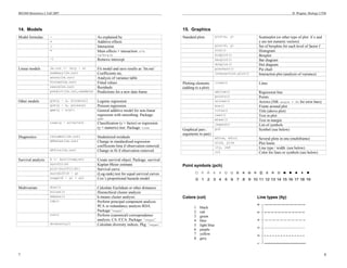
0 1 2 3 4 5 6 7 8 9 10 11 12 13 14 15 16 17 18 19
15. Graphics
Standard plots plot(x, y) Scatterplot (or other type of plot if x and
y are not numeric vectors)
plot(f, y) Set of boxplots for each level of factor f
hist() Histogram
boxplot() Boxplot
barplot() Bar diagram
dotplot() Dot diagram
piechart() Pie chart
interaction.plot() Interaction plot (analysis of variance)
Plotting elements
(adding to a plot)
lines() Lines
abline() Regression line
points() Points
arrows() Arrows (NB: angle = 90 for error bars)
box() Frame around plot
title() Title (above plot)
text() Text in plot
mtext() Text in margin
legend() List of symbols
Graphical pars.:
arguments to par()
pch Symbol (see below)
mfrow, mfcol Several plots in one (multiframe)
xlim, ylim Plot limits
lty, lwd Line type / width (see below)
col Color for lines or symbols (see below)
Point symbols (pch)
Colors (col) Line types (lty)
1 black
2 red
3 green
4 blue
5 light blue
6 purple
7 yellow
8 grey
1
2
3
4
5
6

R Cheat Sheet for Data Analysts and Statisticians.pdf

  • 1.
    BIO360 Biometrics I,Fall 2007 1 R cheat sheet 1. Basics Commands objects() List of objects in workspace ls() Same rm(object) Delete ‘object’ Assignments <- Assign value to a variable = Same Getting help help(fun) Display help file for function fun() args(fun) List arguments of function fun() Libraries / packages library(pkg) Open package (library) ‘pkg’ library(help=pkg) Display description of package ‘pkg’ 2. Vectors and data types Generating seq(-4,4,0.1) Sequence: -4.0, -3.9, -3.8, ..., 3.9, 4.0 2:7 Same as seq(2,7,1) c(5,7,9,1:3) Concatenation (vector): 5 7 9 1 2 3 rep(1,5) 1 1 1 1 1 rep(4:6,1:3) 4 5 5 6 6 6 gl(3,2,12) Factor with 3 levels, repeat each level in blocks of 2, up to length 12 (1 1 2 2 3 3 1 1 2 2 3 3) Coercion as.numeric(x) Convert to numeric as.character(x) Convert to text string as.logical(x) Convert to logical factor(x) Create factor from vector x unlist(x) Convert list, result from table() etc. to vector 3. Data frames Accessing data data.frame(height, weight) Collect vectors ‘height’ and ‘weight’ into data frame dfr&var Select vector ‘var’ in data frame ‘dfr’ attach(dfr) Put data frame in search path detach() - and remove it from the path Editing dfr2 <- edit(dfr) open data frame ‘dfr’ in spreadsheet, write changed version into new data frame ‘dfr2’ fix(dfr) open data frame ‘dfr’ in spreadsheet, changes will overwrite entries in ‘dfr’ Summary dim(dfr) Number of rows and columns in data frame ‘dfr’, works also for matrices and arrays summary(dfr) Summary statistics for each variable in ‘dfr’ H. Wagner, Biology UTM 2 Modified from: P. Dalgaard (2002). Introductory Statistics with R. Springer, New York. 4. Input and export of data General data(name) Built-in data set read.table(“file.txt”) Read from external ASCII file Arguments to read.table() header = TRUE First line has variable names row.names = 1 First column has row names sep = “,” Data are separated by commas sep = “t” Data are separated by tabs dec = “,” Decimal point is comma na.strings = “.” Missing value is dot Variants of read.table() read.csv(“file.csv”) Comma separated read.delim(“file.txt”) Tab delimited text file Export write.table() see help(write.table) for details Adding names names() Column names for data frame or list only dimnames() Row and column names, also for matrix 5. Indexing / selection / sorting Vectors x[1] First element x[1:5] Subvector containing the first five elements x[c(2,3,5)] Elements nos. 2, 3, and 5 x[y <= 30] Selection by logical expression x[sex = = “male”] Selection by factor variable i <-c(2,3,5); x[i] Selection by numerical variable k <- (y <=30); x[k] Selection by logical variable length(x) Returns length of vector x Matrices, data frames m[4, ] Fourth row m[ ,3] Third column drf[drf$var <=30, ] Partial data frame (not for matrices) subset(dfr,var<=30) Same, often simpler (not for matrices) m[m[ ,3]<=30, ] Partial matrix (also for data frames) Sorting sort(c(7,9,10,6)) Returns the sorted values: 6, 7, 9, 10 order(c(7,9,10,6)) Returns the element number in order of ascending values: 4, 1, 2, 3 order(c(7,9,10,6), decreasing = TRUE) same, but in order of decreasing values: 3, 2, 1, 4 rank(c(7,9,10,6)) Returns the ranks in order of ascending values: 2, 3, 4, 1
  • 2.
    BIO360 Biometrics I,Fall 2007 3 6. Missing values Functions is.na(x) Logical vector. TRUE where x has NA complete.cases(x1,x2,...) Neither missing in x1, nor x2, nor ... Arguments to other functions na.rm = In statistical functions: Remove missing if TRUE, returns NA if FALSE na.last = In ‘sort’ TRUE, FALSE and NA means “last”, “first”, and “discard” na.action = in ‘lm()’, etc., values na.fail, na.omit, na.exclude na.print = In ‘summary()’ and ‘print()’: How to represent NA in output na.strings = In ‘read.table()’: Codes(s) for NA in input 7. Numerical functions Mathematical log(x) Logarithm of x, natural logarithm log(x, 10) Base10 logarithm of x exp(x) Exponential function ex sin(x) Sine cos(x) Cosine tan(x) Tangent asin(x) Arcsin (inverse sine) min(x) Smallest value in vector min(x1, x2, ...) minimum number over several vectors max(x) Largest value in vector range(x) Like c(min(x), max(x)) pmin(x1, x2, ...) Parallel (elementwise) minimum over multiple equally long vectors length(x) Number of elements in vector sum(x) Sum of values in vector cumsum(x) Cumulative sum of values in vector sum(complete.cases(x)) Number of non-missing elements Statistical mean(x) Average median(x) Median quantile(x, p) Quantiles: median = quantile(x, 0.5) var(x) Variance sd(x) Standard deviation cor(x, y) Pearson correlation cor(x, y, method = “spearman”) Spearman rank correlation H. Wagner, Biology UTM 4 8. Programming Conditional execution if(p< 0.5) print(“Hooray”) Print “Hooray” if condition is true if(p < 0.5) { print(“Hooray”) i = i + 1 } If condition is true, perform all commands within the curved brackets { } if(p < 0.5) { print(“Hooray”)} else { i = i + 1} Conditional execution with an alternative Loop for(i in 1:10) { print(i) } Go through loop 10 times i <- 1 while(i <= 10) { print(i) i = i + 1 } Same, but more complicated User-defined function fun<- function(a, b, doit = FALSE) { if(doit) {a + b} else 0 } Defines a function ‘fun’ that returns the sum of a and b if the argument ‘doit’ is set to TRUE, or zero, if ‘doit’ is FALSE 9. Operators Arithmetic + Addition - Subtraction * Multiplication / Division ^ Raise to the power of % / % Integer division: 5 %/% 3 = 1 % % Remainder from integer division: 5 %% 3 = 2 Logical or relational = = Equal to ! = Not equal to < Less than > Greater than < = Less than or equal to > = Greater than or equal to is.na(x) Missing? & Logical AND | Logical OR ! Logical NOT
  • 3.
    BIO360 Biometrics I,Fall 2007 5 10. Tabulation, grouping, recoding General table(x) Frequency table of vector (factor) x table(x, y) Crosstabulation of x and y xtabs(~ x + y) Formula interface for crosstabulation: use summary() for chi-square test factor(x) Convert vector to factor cut(x, breaks) Groups from cutpoints for continuous variable, breaks is a vector of cutpoints Arguments to factor() levels = c() Values of x to code. Use if some values are not present in data, or if the order would be wrong. labels = c() Values associated with factor levels exclude = c() Values to exclude. Default NA. Set to NULL to have missing values included as a level. Arguments to cut() breaks = c() Cutpoints. Note values of x outside of ‘breaks’ gives NA. Can also be a single number, the number of cutpoints. labels = c() Names for groups. Default is 1, 2, ... Factor recoding levels(f) <- names New level names factor(newcodes[f]) Combining levels: ‘newcodes’, e.g., c(1,1,1,2,3) to amalgamate the first 3 of 5 groups of factor f 11. Manipulations of matrices and lists Matrix algebra m1 % * % m2 Matrix product t(m) Matrix transpose m[lower.tri(m)] Returns the values from the lower triangle of matrix m as a vector diag(m) Returns the diagonal elements of matrix m matrix(x, dim1, dim2) Fill the values of vector x into a new matrix with dim1 rows and dim2 columns, Marginal operations etc. apply(m, dim, fun) Applies the function ‘fun’ to each row (dim = 1) or column (dim= 2) of matrix m tapply(m, list(f1, f2), fun) Can be used to aggregate columns or rows within matrix m as defined by f1, f2, using the function ‘fun’ (e.g., mean, max) split(x, f) Split vector, matrix or data frame by factor x. Different results for matrix and data frame! The result is a list with one object for each level of f. sapply(list, fun) sapply(split(x,f), fun) applies the function ‘fun’ to each object in a list, e.g. as created by the split function H. Wagner, Biology UTM 6 12. Statistical standard methods Parametric tests, continuous data t.test One- and two-sample t-test pairwise.t.test Pairwise comparison of means cor.test Significance test for correlation coeff. var.test Comparison of two variances (F-test) lm(y ~ x) Regression analysis lm(y ~ f) One-way analysis of variance lm(y ~ x1 + x2 + x3) Multiple regression lm(y ~ f1 * f2) Two-way analysis of variance Non-parametric wilcox.test One- and two-sample Wilcox test kruskal.test Kruskal-Wallis test friedman.test Friedman’s two-way analysis of variance cor.test variant method = “spearman” Spearman rank correlation Discrete response binom.test Binomial test (incl. sign test) prop.test Comparison of proportions fisher.test Exact test in 2 x 2 tables chisq.test Chi-square test of independence glm(y ~ x1+x2, binomial) Logistic regression 13. Statistical distributions Normal distribution dnorm(x) Density function pnorm(x) Cumulative distribution function P(X<=x) qnorm(p) p-quantile, returns x in: P(X<=x) = p rnorm(n) n random normally distributed numbers Distributions pnorm(x, mean, sd) Normal plnorm*x, mean, sd) Lognormal pt(x, df) Student’s t distribution pf(x, n1, n2) F distribution pchisq(x, df) Chi-square distribution pbinom(x, n, p) Binomial ppois(x, lambda) Poisson punif(x, min, max) Uniform pexp(x, rate) Exponential pgamma(x, shape, scale) Gamma pbeta(x, a, b) Beta
  • 4.
    BIO360 Biometrics I,Fall 2007 7 14. Models Model formulas ~ As explained by + Additive effects : Interaction * Main effects + interaction: a*b =a+b+a:b -1 Remove intercept Linear models lm.out <- lm(y ~ x) Fit model and save results as ‘lm.out’ summary(lm.out) Coefficients etc. anova(lm.out) Analysis of variance table fitted(lm.out) Fitted values resid(lm.out) Residuals predict(lm.out,newdata) Predictions for a new data frame Other models glm(y ~ x, binomial) Logistic regression glm(y ~ x, poisson) Poisson regression gam(y ~ s(x)) General additive model for non-linear regression with smoothing. Package: gam tree(y ~ x1+x2+x3) Classification (y = factor) or regression (y = numeric) tree. Package: tree Diagnostics rstudent(lm.out) Studentized residuals dfbetas(lm.out) Change in standardized regression coefficients beta if observation removed dffits(lm.out) Change in fit if observation removed Survival analysis S <- Surv(time,ev) Create survival object. Package: survival survfit(S) Kaplan-Meier estimate plot(survfit(S)) Survival curve survdiff(S ~ g) (Log-rank) test for equal survival curves coxph(S ~ x1 + x2) Cox’s proportional hazards model Multivariate dist() Calculate Euclidean or other distances hclust() Hierarchical cluster analysis kmeans() k-means cluster analysis rda() Perform principal component analysis PCA or redundancy analysis RDA. Package ‘vegan’. cca() Perform (canonical) correspondence analysis, CA /CCA. Package: ‘vegan’ diversity() Calculate diversity indices. Pkg: ‘vegan’ H. Wagner, Biology UTM 8 0 1 2 3 4 5 6 7 8 9 10 11 12 13 14 15 16 17 18 19 15. Graphics Standard plots plot(x, y) Scatterplot (or other type of plot if x and y are not numeric vectors) plot(f, y) Set of boxplots for each level of factor f hist() Histogram boxplot() Boxplot barplot() Bar diagram dotplot() Dot diagram piechart() Pie chart interaction.plot() Interaction plot (analysis of variance) Plotting elements (adding to a plot) lines() Lines abline() Regression line points() Points arrows() Arrows (NB: angle = 90 for error bars) box() Frame around plot title() Title (above plot) text() Text in plot mtext() Text in margin legend() List of symbols Graphical pars.: arguments to par() pch Symbol (see below) mfrow, mfcol Several plots in one (multiframe) xlim, ylim Plot limits lty, lwd Line type / width (see below) col Color for lines or symbols (see below) Point symbols (pch) Colors (col) Line types (lty) 1 black 2 red 3 green 4 blue 5 light blue 6 purple 7 yellow 8 grey 1 2 3 4 5 6