R is an open source statistical programming language and software environment used widely for statistical analysis and graphics. This document provided an introduction to using R, including downloading and installing R, the basic R environment and interface, help resources, loading and using packages, reading data into R from files, and performing common descriptive statistics and linear regression modeling. Examples were provided using built-in and example datasets to demonstrate summarizing data, exploring variables, and fitting simple statistical models in R.

1. ‫البحث‬ ‫أدوات‬ ‫سلسلة‬‫العلمي‬(1)
‫عمل‬ ‫شة‬‫ر‬‫و‬«‫الكمي‬ ‫التحليل‬ ‫برنامج‬R Program»
‫والطبية‬ ‫العلمية‬ ‫الدراسات‬ ‫بحوث‬ ‫مركز‬
‫سعود‬ ‫الملك‬ ‫جامعة‬

2. An Introduction to R-
Programming
Hadeel Alkofide, Msc, PhD
NOT a biostatistician or R expert just simply an R user
Some slides were adapted from lectures by
Angie Mae Rodday MSc, PhD at Tufts University

3. What is R?
• Open source programming language and software
environment for statistical computing and graphics
• R is an implementation of the S programming language
• S was created by John Chambers while at Bell Labs
• R was created by Ross Ihaka and Robert Gentleman
• R is named partly after the first names of the first two R
authors and partly as a play on the name of S

4. • FREE and Open Source
• Strong user Community
• Highly extensible, flexible
• Implementation of high end statistical methods
• Flexible graphics and intelligent defaults
• Runs on Windows, Mac OS, and Linux/UNIX platforms
Why Use R?

5. • Difficult, but NOT FOR YOU ☺
• Command- (not menu-) driven.
• No commercial support, means you need to look for
solutions your self, which can be very frustrating
• Easy to make mistakes and not know
• Data prep and cleaning can be messier and more
mistake prone in R vs. SPSS or SAS
Then, why is not everyone using R???

6. Survey Asking Researched their Primary Data
Analysis Tool?
https://r4stats.wordpress.com/articles/popularity/

7. Let us start learning R

8. Learning R… Piece of cake

9. Downloading R
• https://cran.r-project.org/

10. The R Environment- R Command Window

11. • R command window (console) or Graphical User
Interface (GUI)
• Used for entering commands, data manipulations,
analyses, graphing
• Output: results of analyses, queries, etc. are written
here
• Toggle through previous commands by using the up
and down arrow keys
The R Environment- R Command Window

12. The R Environment- R Command Window
The prompt ‘>’ indicates that R is your commands
R is case sensitive (y ≠ Y)
In the Console, use the up and down arrows to scroll
back to previous code

13. • Current working environment
• Comprised primarily of variables, datasets, functions
The R Environment- R Workspace

14. • 2+2
• 2*2
• 2*100/2
• 2^10
• 2*5^2
• X<-2*5^2
• X
R as Calculator
In R <- indicates that you making an assignment. This
will come up often, particularly with data manipulation

15. Operations in R
Comparison
operators
Purpose Example
== Equal 1==1 returns TRUE
!= Not equal 1!=1 returns FALSE
< > Great/less than 1<1 returns FALSE
>= <= Greater/less than or equal 1<=1 returns TRUE
Logical operators
& And—must meet both condition 1==1 & 1<1 returns FALSE
| (above backslash
key)
Or—only needs to meet 1
condition
1==1 | 1<1 returns TRUE

16. • A text file containing commands that you would enter
on the command line of R
• To place a comment in a R script, use a hash mark (#)
at the beginning of the line
The R Environment- R Script

17. • In the R console, you can create a new script (from the
file menu → “New Script”) and write all of your R code
there
• This allows you to save your code (but not output) for
later
• To place a comment in a R script, use a hash mark (#)
at the beginning of the line
The R Environment- R Script

18. The R Environment- R Script

19. The R Environment- R Script

20. The R Environment- R Script

21. • When working from your script, you can highlight
sections of code and press “F5” to automatically get
the code to run in the R console
• When saving your script, type the extension “.R” after
the file name so that your computer recognizes that it is
an R file (e.g., Hadeel.R)
• You can then open previously saved scripts to re-run or
modify your code
The R Environment- R Script

22. • Saving output using R’s menu options can be annoying
• One option is to copy and paste (into a Word document) the output
that you need while working
• Problem with waiting until the end:
➢ You end up copying a bunch of code and output you may not
need (e.g., you’ll be copying all your errors)
➢ At some point, the R console window fills up and you can’t
access your earlier work
• When copying and pasting your R output, you can change the font to
“Courier New” and the output will line up and look pretty
Saving Output (Results)

23. • Everything that you work within R is an object
• Types of objects include vectors, matrices, and data
frames
• To see which objects are available in the “workspace”
(i.e., R memory) use the command ls() or objects()
• You can remove objects with the rm()function
• The class() function tells you the type of object
Objects in R

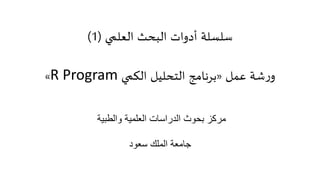
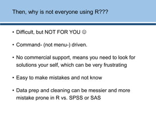
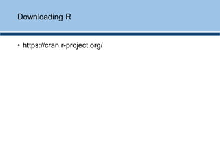
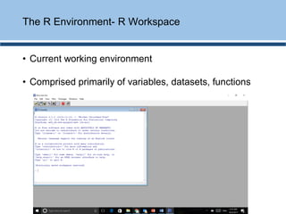
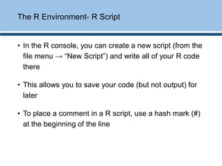
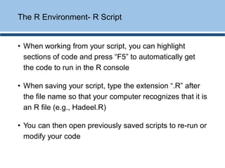
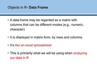
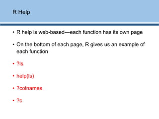
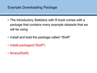
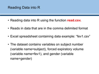
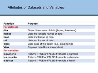
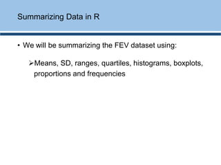
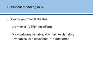
24. • An ordered collection of numerical, categorical,
complex or logical objects
• vec1<-1:10
• vec1
• [1] 1 2 3 4 5 6 7 8 9 10
• class(vec1)
• [1] "integer"
Objects in R- Vectors
This is putting numbers 1
through 10 into a vector
called, “vec1”

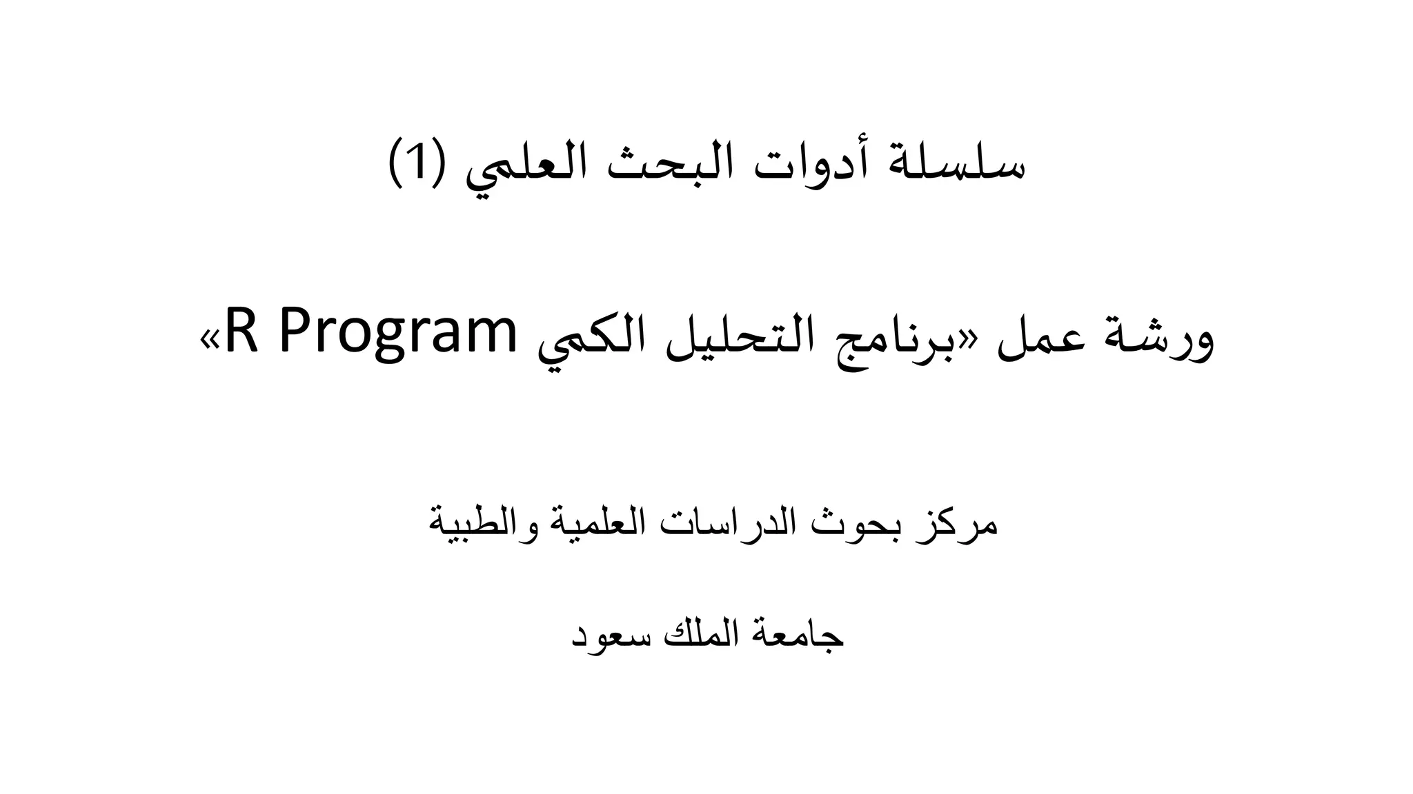
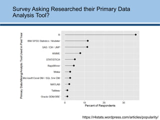
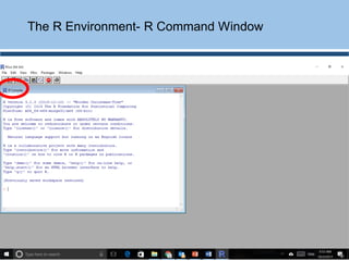
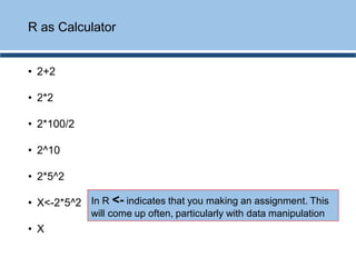
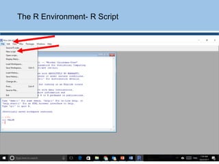
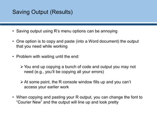
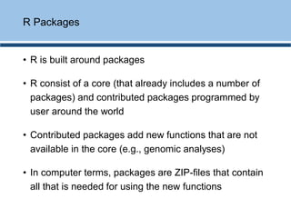
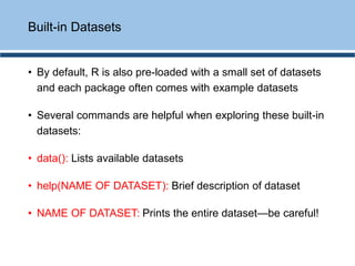
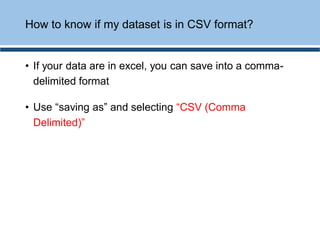
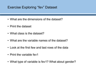
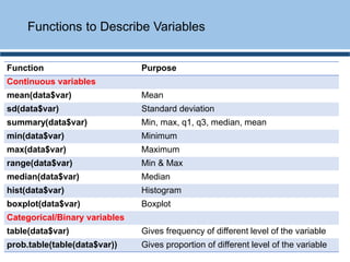
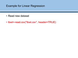
25. • vec2<-LETTERS[1:10]
• vec2
• [1] "A" "B" "C" "D" "E" "F" "G" "H" "I" "J“
• class(vec2)
• [1] "character"
Objects in R- Vectors
This is putting letters A (1st
letter) through J (10th letter)
into a vector called, “vec2”

26. • A matrix is a multidimensional collection of data entries
of the same type
• Matrices have two dimensions: rows and columns
• mat1 <- matrix(vec1, ncol = 2, nrow = 5)
Objects in R- Matrix
Function to create
a matrix
What will be going into the matrix
(we are putting vec1 that we
created above into the matrix)
Number of columns
in the matrix
Number of rows in
the matrix

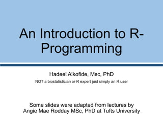
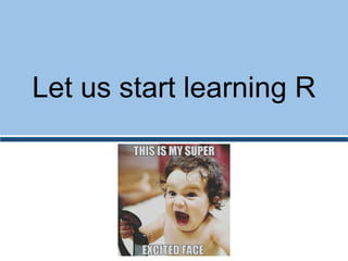
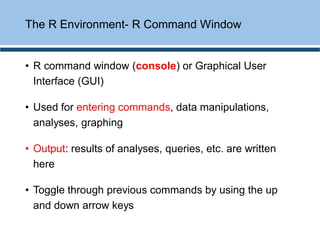
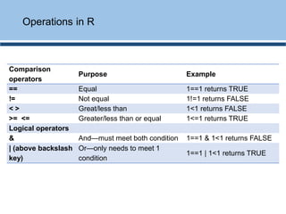
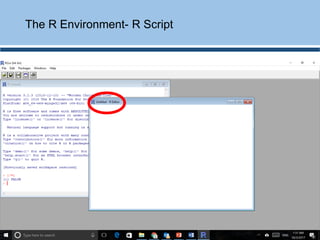
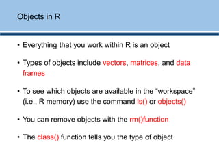
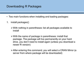
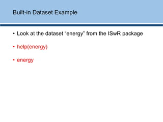
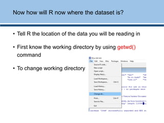
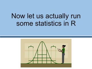
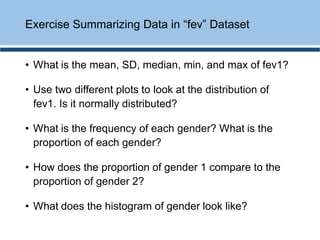
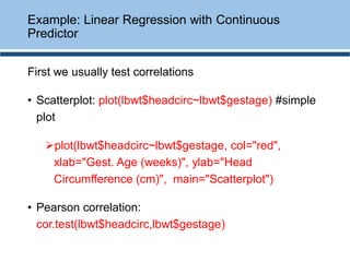
27. • mat1 <- matrix(vec1, ncol = 2, nrow = 5)
• class(mat1)
• [1] "matrix"
Objects in R- Matrix
[,1] [,2]
[1,] 1 6
[2,] 2 7
[3,] 3 8
[4,] 4 9
[5,] 5 10

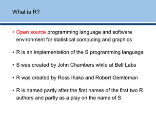
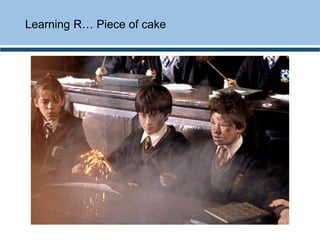
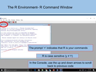
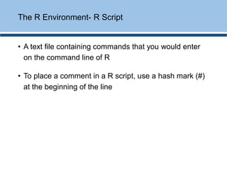
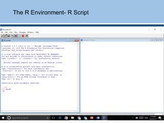
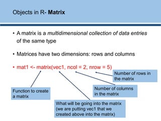
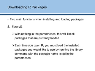
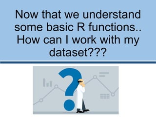
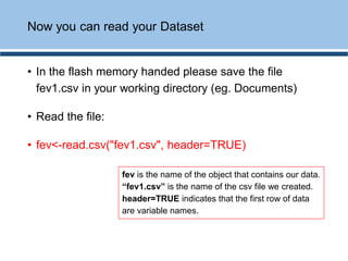
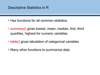
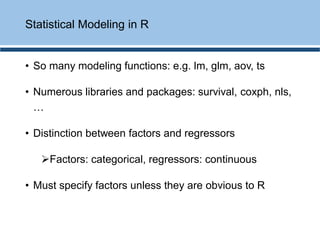
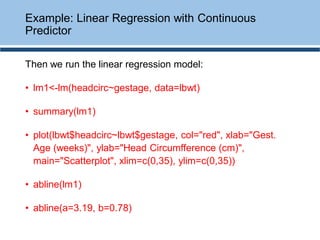
28. • To find the dimensions (i.e., number of rows and
columns) of the matrix:
• dim(mat1)
• [1] 5 2
• Print the data in the first row of the matrix:
• mat1[1,]
• [1] 1 6
Objects in R- Matrix

29. • A data.frame may be regarded as a matrix with
columns that can be different modes (e.g., numeric,
character)
• It is displayed in matrix form, by rows and columns
• It’s like an excel spreadsheet
• This is primarily what we will be using when analyzing
our data in R
Objects in R- Data Frame

30. • Creates a data frame from the matrix we had
previously made:
• df1<-data.frame(mat1)
• df1
Objects in R- Data Frame

31. Objects in R- Data Frame
Find class of the dataframe
Find dimension of the dataframe
Print first row of the dataframe
Print first column of the dataframe
Find class of the dataframe

32. Objects in R- Let’s Play a little with the Data Frame
When
referring
to a
variable
within a
data
frame,
you must
use the
$ sign
Print data for variable “X1”
Take the mean of variable X2 in the data frame
Assign the name “var1” to the first variable X1 and
“var2” to the second variable X2
Review the objects that we have created

33. • R help is web-based—each function has its own page
• On the bottom of each page, R gives us an example of
each function
• ?ls
• help(ls)
• ?colnames
• ?c
R Help

34. • R is built around packages
• R consist of a core (that already includes a number of
packages) and contributed packages programmed by
user around the world
• Contributed packages add new functions that are not
available in the core (e.g., genomic analyses)
• In computer terms, packages are ZIP-files that contain
all that is needed for using the new functions
R Packages

35. • Two main functions when installing and loading packages:
1. install.packages()
➢With nothing in parentheses: list all packages available to
install
➢With the name of package in parentheses: install that
package. The package will live permanently on your hard
drive, you don’t need to install again (unless you download a
newer R version)
➢After entering this command, you will select a CRAN Mirror (a
server from where package will be downloaded)
Downloading R Packages

36. • Two main functions when installing and loading packages:
2. library()
➢With nothing in the parentheses, this will list all
packages that are currently loaded
➢Each time you open R, you must load the installed
packages you would like to use by running the library
command with the package name listed in the
parentheses
Downloading R Packages

37. • The Introductory Statistics with R book comes with a
package that contains many example datasets that we
will be using
• Install and load the package called “ISwR”
• install.packages("ISwR")
• library(ISwR)
Example Downloading Package

38. • By default, R is also pre-loaded with a small set of datasets
and each package often comes with example datasets
• Several commands are helpful when exploring these built-in
datasets:
• data(): Lists available datasets
• help(NAME OF DATASET): Brief description of dataset
• NAME OF DATASET: Prints the entire dataset—be careful!
Built-in Datasets

39. • Look at the dataset “energy” from the ISwR package
• help(energy)
• energy
Built-in Dataset Example

40. Now that we understand
some basic R functions..
How can I work with my
dataset???

41. • Reading data into R using the function read.csv.
• Reads in data that are in the comma delimited format
• Excel spreadsheet containing data example: “fev1.csv”
• The dataset contains variables on subject number
(variable name=subject), forced expiratory volume
(variable name=fev1), and gender (variable
name=gender)
Reading Data into R

42. • If your data are in excel, you can save into a comma-
delimited format
• Use “saving as” and selecting “CSV (Comma
Delimited)”
How to know if my dataset is in CSV format?

43. • Tell R the location of the data you will be reading in
• First know the working directory by using getwd()
command
• To change working directory
Now how will R now where the dataset is?

44. • In the flash memory handed please save the file
fev1.csv in your working directory (eg. Documents)
• Read the file:
• fev<-read.csv("fev1.csv", header=TRUE)
Now you can read your Dataset
fev is the name of the object that contains our data.
“fev1.csv” is the name of the csv file we created.
header=TRUE indicates that the first row of data
are variable names.

45. Function Purpose
For datasets
dim Gives dimensions of data (#rows, #columns)
names Lists the variable names of data
head Lists first 6 rows of data
tail Lists last 6 rows of data
class Lists class of the object (e.g., data frame)
View Displays data like a spreadsheet
For variables
is.numeric Returns TRUE or FALSE if variable is numeric
is.character Returns TRUE or FALSE if variable is character
is.factor Returns TRUE or FALSE if variable is factor
Attributes of Datasets and Variables

46. • What are the dimensions of the dataset?
• Print the dataset
• What class is the dataset?
• What are the variable names of the dataset?
• Look at the first few and last rows of the data
• Print the variable fev1
• What type of variable is fev1? What about gender?
Exercise Exploring “fev” Dataset

47. Now let us actually run
some statistics in R

48. • Has functions for all common statistics
• summary() gives lowest, mean, median, first, third
quartiles, highest for numeric variables
• table() gives tabulation of categorical variables
• Many other functions to summarize data
Descriptive Statistics in R

49. • We will be summarizing the FEV dataset using:
➢Means, SD, ranges, quartiles, histograms, boxplots,
proportions and frequencies
Summarizing Data in R

50. Function Purpose
Continuous variables
mean(data$var) Mean
sd(data$var) Standard deviation
summary(data$var) Min, max, q1, q3, median, mean
min(data$var) Minimum
max(data$var) Maximum
range(data$var) Min & Max
median(data$var) Median
hist(data$var) Histogram
boxplot(data$var) Boxplot
Categorical/Binary variables
table(data$var) Gives frequency of different level of the variable
prob.table(table(data$var)) Gives proportion of different level of the variable
Functions to Describe Variables

51. • What is the mean, SD, median, min, and max of fev1?
• Use two different plots to look at the distribution of
fev1. Is it normally distributed?
• What is the frequency of each gender? What is the
proportion of each gender?
• How does the proportion of gender 1 compare to the
proportion of gender 2?
• What does the histogram of gender look like?
Exercise Summarizing Data in “fev” Dataset

52. • So many modeling functions: e.g. lm, glm, aov, ts
• Numerous libraries and packages: survival, coxph, nls,
…
• Distinction between factors and regressors
➢Factors: categorical, regressors: continuous
• Must specify factors unless they are obvious to R
Statistical Modeling in R

53. • Specify your model like this:
➢y ~ xi+ci (VERY simplified)
➢y = outcome variable, xi = main explanatory
variables, ci = covariates, + = add terms
Statistical Modeling in R

54. • Read new dataset
• lbwt<-read.csv("lbwt.csv", header=TRUE)
Example for Linear Regression

55. First we usually test correlations
• Scatterplot: plot(lbwt$headcirc~lbwt$gestage) #simple
plot
➢plot(lbwt$headcirc~lbwt$gestage, col="red",
xlab="Gest. Age (weeks)", ylab="Head
Circumfference (cm)", main="Scatterplot")
• Pearson correlation:
cor.test(lbwt$headcirc,lbwt$gestage)
Example: Linear Regression with Continuous
Predictor

56. Then we run the linear regression model:
• lm1<-lm(headcirc~gestage, data=lbwt)
• summary(lm1)
• plot(lbwt$headcirc~lbwt$gestage, col="red", xlab="Gest.
Age (weeks)", ylab="Head Circumfference (cm)",
main="Scatterplot", xlim=c(0,35), ylim=c(0,35))
• abline(lm1)
• abline(a=3.19, b=0.78)
Example: Linear Regression with Continuous
Predictor

57. How to Learn More
About R?

58. • R home page: http://www.r-project.org
• R discussion group:
http://www.stat.math.ethz.ch/mailman/listinfo/r-help
• Search Google for R and Statistics
R Resources

59. • http://www.statmethods.net/stats/
• http://scc.stat.ucla.edu/mini-courses
• http://www.ats.ucla.edu/stat/R/
Tutorials

60. • http://www.datasciencecentral.com/profiles/blogs/10-
great-books-about-r-1
Top 10 Great Books About R

61. Thank you