The document discusses the intersection of information retrieval (IR) and quantum probabilities, presenting a framework that combines geometry, probability, and logic within IR models. It covers the basics of quantum formalism, including Hilbert spaces and linear operators, and how these concepts can be applied to develop quantum-inspired IR models. The paper acknowledges previous works and tutorials on this topic while providing a foundation for further exploration of quantum mechanics in information retrieval.

1. The Geometry of Information Retrieval
Quantum Probabilities and Quantum-inspired IR Models
Ingo Frommholz
University of Bedfordshire
Luton, UK
ingo.frommholz@beds.ac.uk
Herbstschule Information Retrieval
Schloss Dagstuhl

2. Table of Contents
1 Introduction
2 Introduction to Quantum Probabilities
3 Quantum-inspired IR Models
4 Further Models and Conclusion
2 / 145

3. Acknowledgements
Some parts (in particular the quantum probability one) are based
on the ECIR 2012 “Quantum Information Access and Retrieval”
tutorial given by Benjamin Piwowarski and Massimo Melucci
This tutorial is worth checking out
It covers some aspect more thoroughly
It discusses some further quantum-based IR models
See also
http://www.bpiwowar.net/2012/04/
slides-from-the-ecir12-quantum-information-access-and-retrieval-tutorial/
Direct download:
http://www.bpiwowar.net/wp-content/uploads/2012/04/tutorial-handout.pdf
I’d like to thank Guido Zuccon for providing material about qPRP
3 / 145

4. Introduction
IR and Geometry

5. Introduction
IR and Geometry
IR Models and Principles
Geometry, Probability and Logics
VSM LSI
QIA
qPRP QM
pDatalog
LUP
LM iPRP Boolean
BM25
PRP
5 / 145

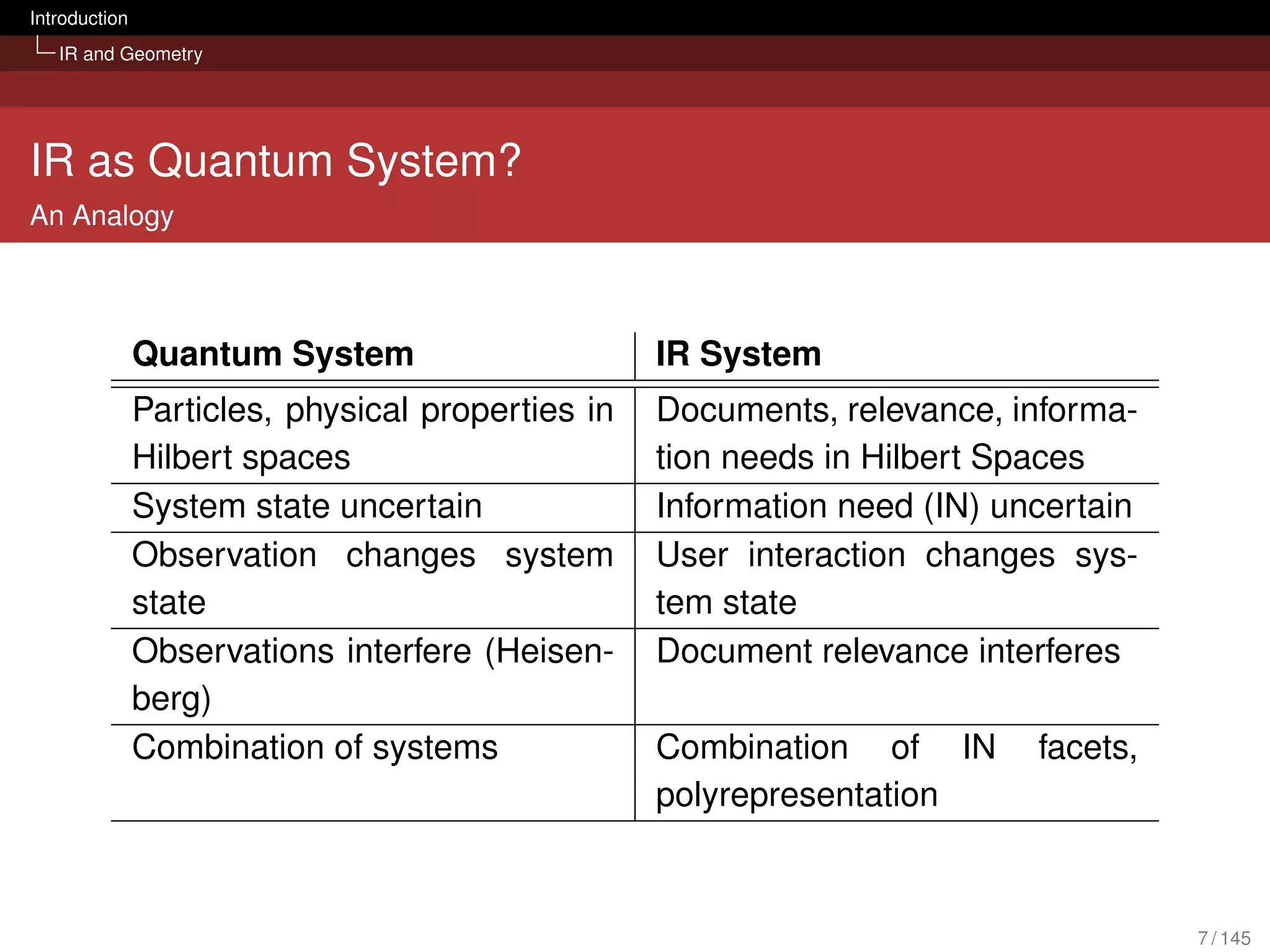
6. Introduction
IR and Geometry
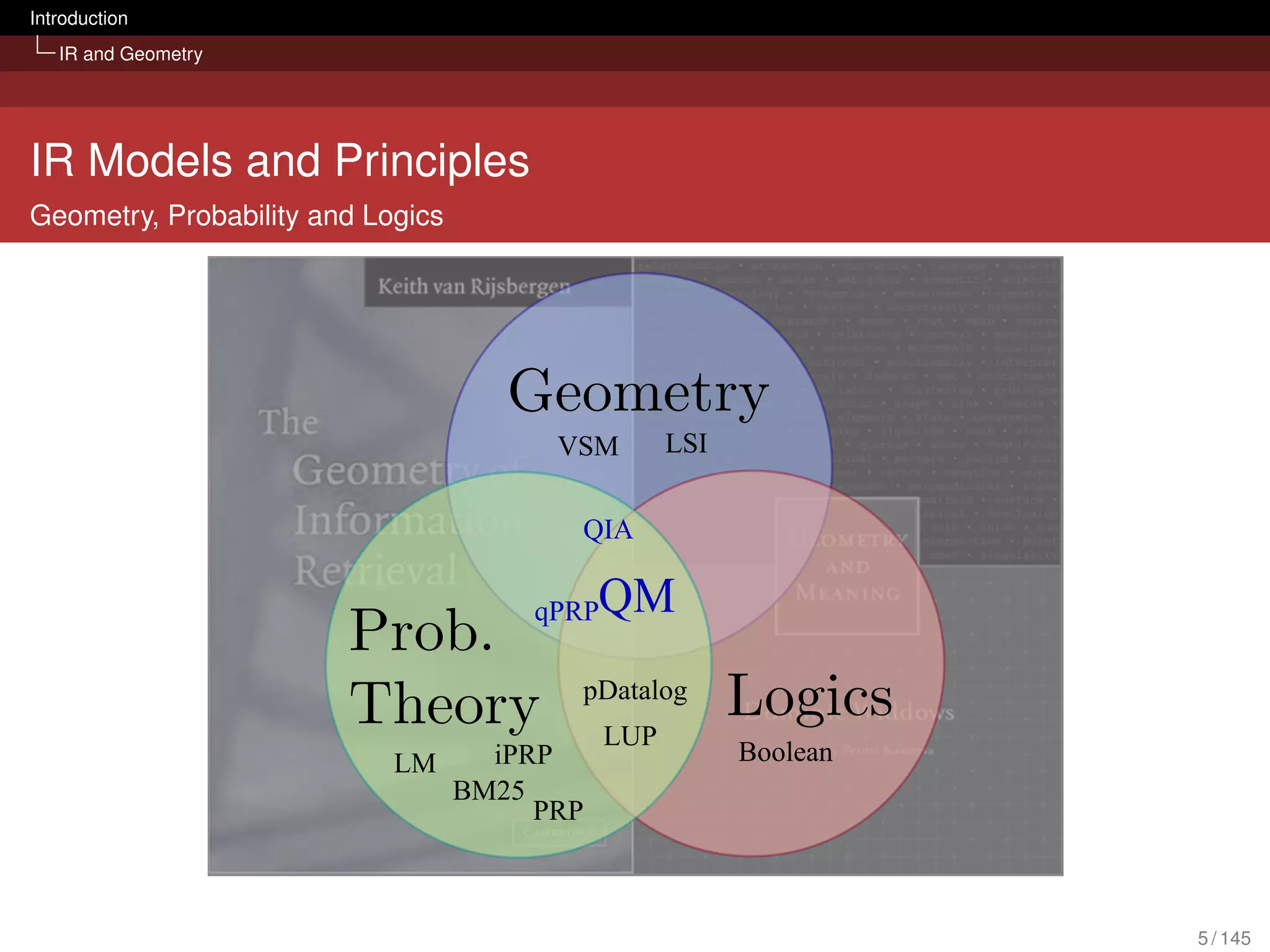
A Language for IR
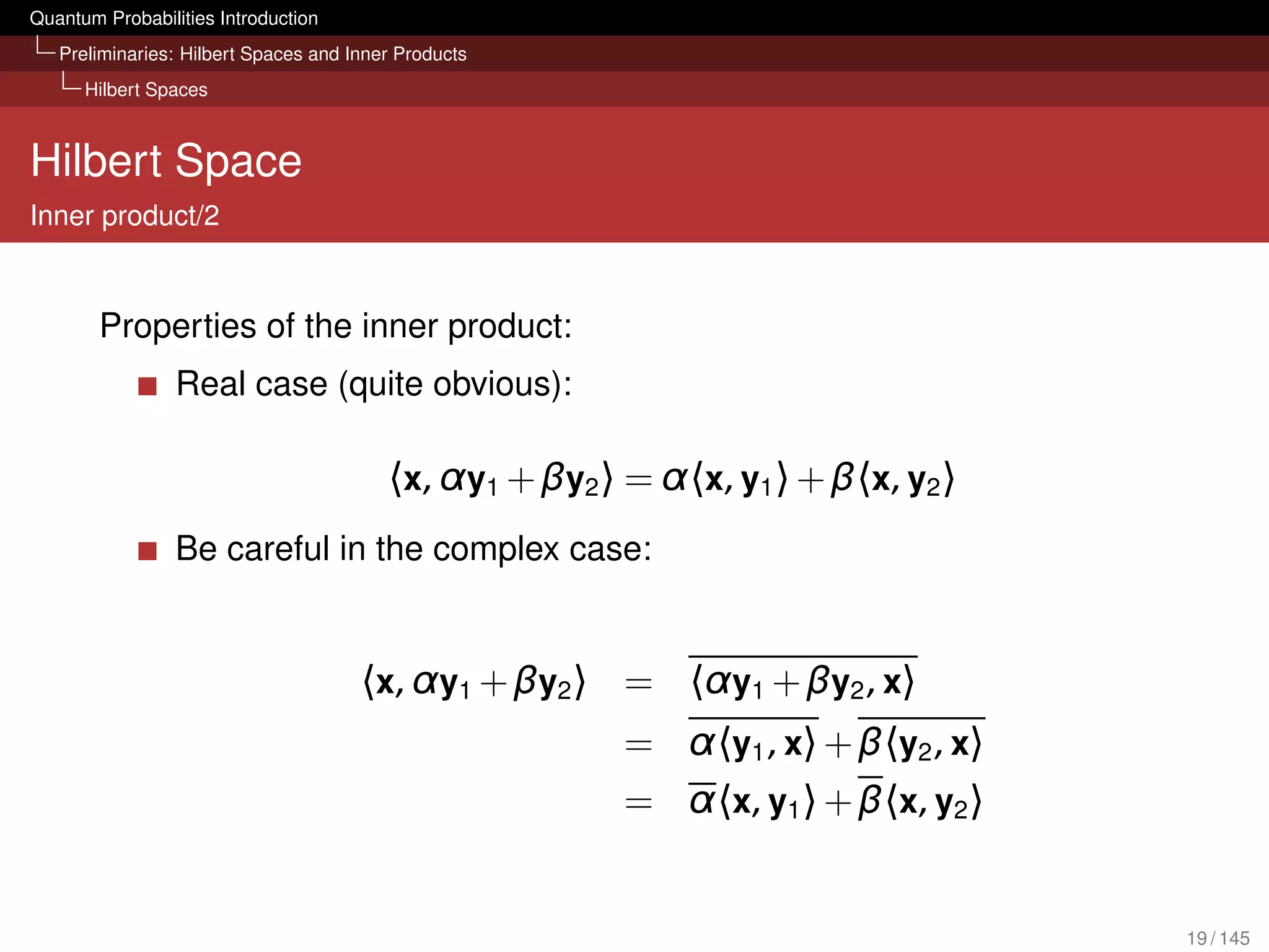
The geometry and mathematics behind quantum mechanics can
be seen as a ’language’ for expressing the different IR models
[van Rijsbergen, 2004].
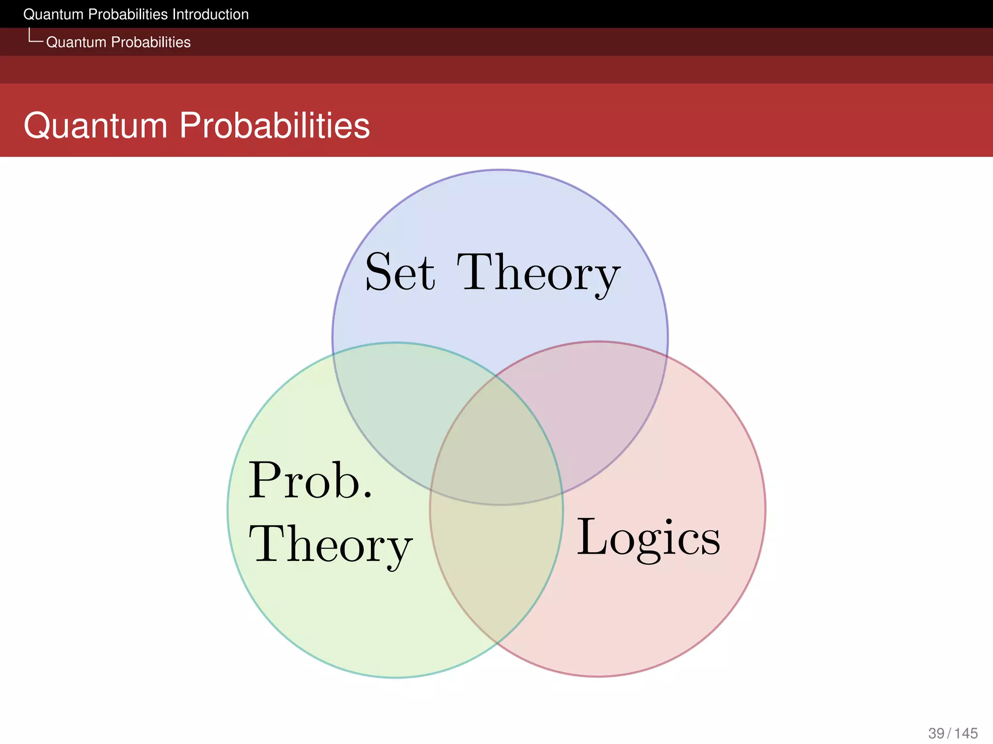
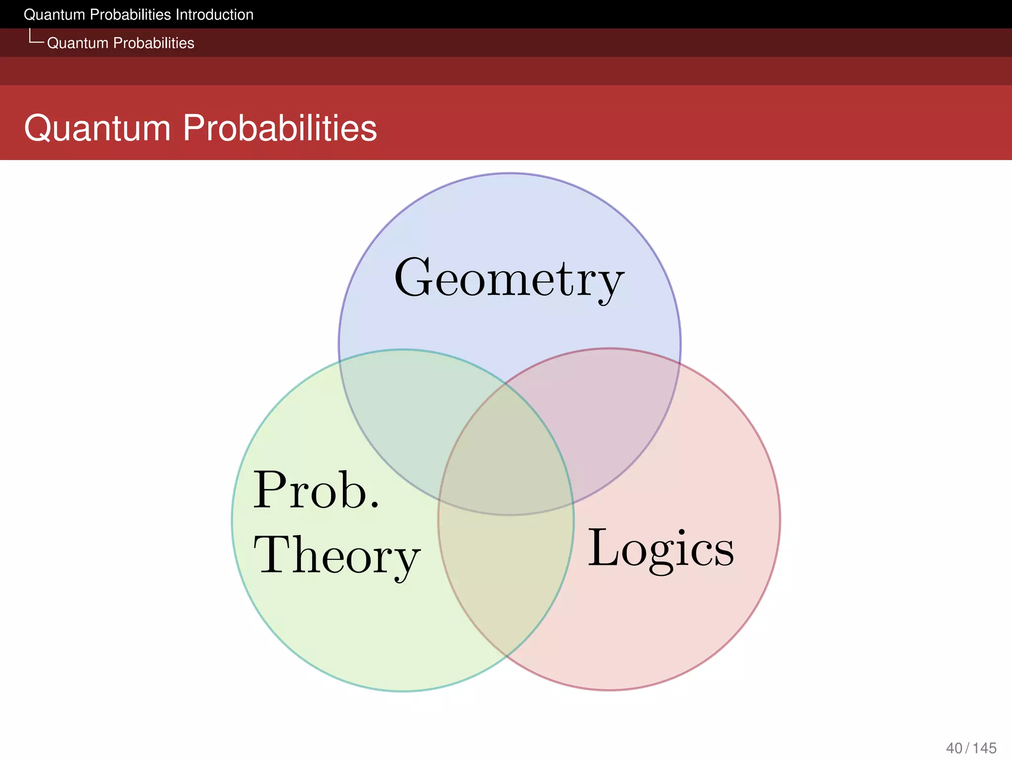
Combination of geometry, probability and logics
Leading to non-classical probability theory and logics
Potential unified framework for IR models
Applications in areas outside physics emerging
Quantum Interaction symposia (e.g. [Song et al., 2011])
6 / 145

7. Introduction
IR and Geometry
IR as Quantum System?
An Analogy
Quantum System IR System
Particles, physical properties in Documents, relevance, informa-
Hilbert spaces tion needs in Hilbert Spaces
System state uncertain Information need (IN) uncertain
Observation changes system User interaction changes sys-
state tem state
Observations interfere (Heisen- Document relevance interferes
berg)
Combination of systems Combination of IN facets,
polyrepresentation
7 / 145

8. Introduction
IR and Geometry
Brief History of the Quantum Formalism
1890s Max Planck’s hypothesis: energy not continuous but
comes in quantas
1920s Born/Jordan: matrix reformulation of Heisenberg’s work
1930s Dirac/von Neumann: mathematical formulation of
quantum physics (Hilbert space), theory of quantum
measurement, quantum logics
8 / 145

9. Introduction to Quantum Probabilities
Quantum Formalism
Preliminaries: Hilbert Spaces and Inner Products
Complex Numbers
Hilbert Spaces
Operators and Projectors
Tensor Spaces
Quantum Probabilities
Quantum and Classical Probabilities
Dirac Notation
Events
Quantum Logics
Quantum States
Pure States
Mixed States
Density Operators
Conclusion

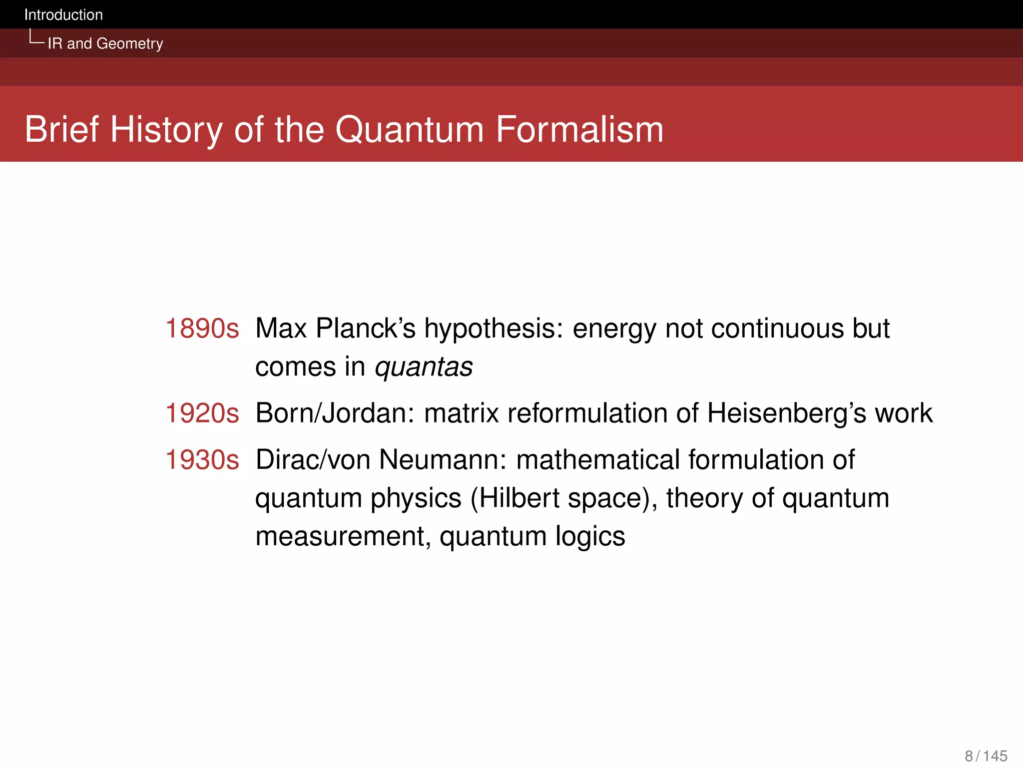
10. Quantum Probabilities Introduction
Quantum Formalism
Quantum Formalism
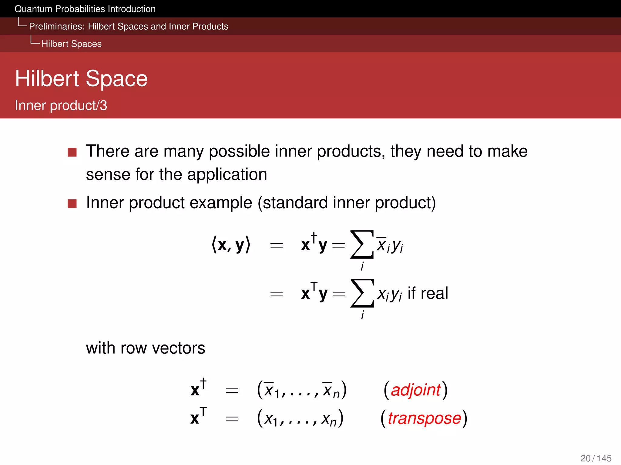
The quantum formalism is build on top of Hilbert spaces
Each finite-dimensional vector space with an inner product is a
Hilbert space [Halmos, 1958]
We focus on finite-dimensional spaces here
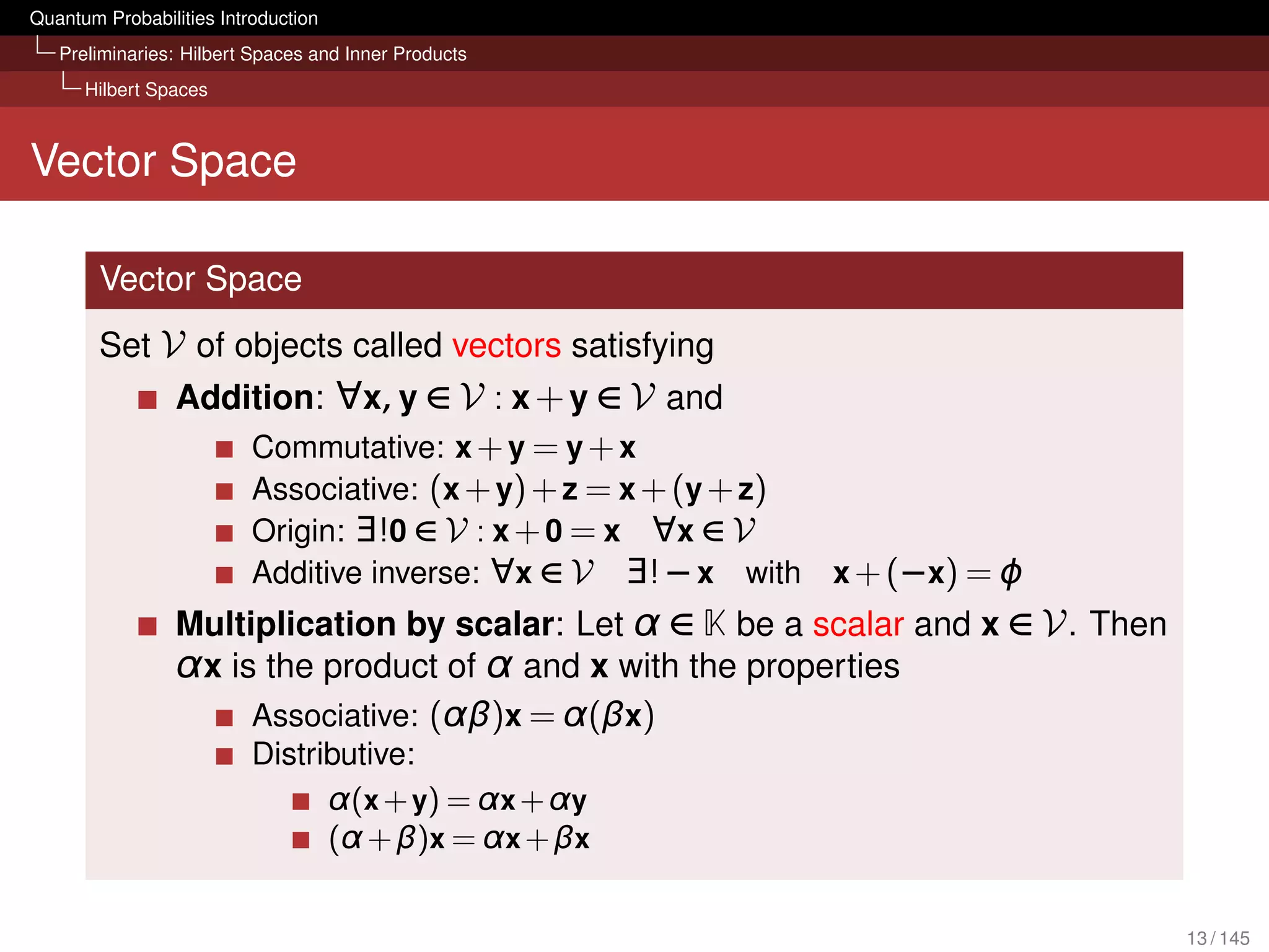
A vector space is defined over a field K, e.g R or C
10 / 145

11. Quantum Probabilities Introduction
Preliminaries: Hilbert Spaces and Inner Products
Complex Numbers
Complex Numbers
Complex number z ∈ C
z = a + ib, a, b ∈ R, i2 = −1
Polar form: z =
r (cos(φ) + i sin(φ)) = reiφ
with r ∈ R+ , φ ∈ [0, 2π]
Addition/Multiplication:
z1 = a1 + ib1 = r1 eiφ1 ,
z2 = a2 + ib2 = r2 eiφ2 :
z1 + z2 = (a1 + a2 )+ i (b1 + b2 )
z1 · z2 = r1 r2 ei(φ1 +φ2 )
11 / 145

12. Quantum Probabilities Introduction
Preliminaries: Hilbert Spaces and Inner Products
Complex Numbers
Complex Numbers
Complex number z ∈ C
z = a + ib, a, b ∈ R, i2 = −1
Polar form: z =
r (cos(φ) + i sin(φ)) = reiφ
with r ∈ R+ , φ ∈ [0, 2π]
Complex conjugate
z = a − ib = re −iφ
b = 0 ⇔z ∈ R ⇔z = z
Absolute value
| z | = a2 + b 2 = r = zz
|z |2 = zz
12 / 145

13. Quantum Probabilities Introduction
Preliminaries: Hilbert Spaces and Inner Products
Hilbert Spaces
Vector Space
Vector Space
Set V of objects called vectors satisfying
Addition: ∀x, y ∈ V : x + y ∈ V and
Commutative: x + y = y + x
Associative: (x + y) + z = x + (y + z)
Origin: ∃!0 ∈ V : x + 0 = x ∀x ∈ V
Additive inverse: ∀x ∈ V ∃! − x with x + (−x) = ϕ
Multiplication by scalar: Let α ∈ K be a scalar and x ∈ V . Then
α x is the product of α and x with the properties
Associative: (αβ)x = α(βx)
Distributive:
α(x + y) = α x + α y
(α + β)x = α x + βx
13 / 145

14. Quantum Probabilities Introduction
Preliminaries: Hilbert Spaces and Inner Products
Hilbert Spaces
Vector Space
Example
Example: n-dimensional complex vector space Cn :
 
x
 .1 
x= . 
 . 
xn
with xi ∈ C and
   
x +y α x1
 1 . 1  . 
. . 

x+y = 

.
 and
 αx = 
 . 
xn + yn α xn
14 / 145

15. Quantum Probabilities Introduction
Preliminaries: Hilbert Spaces and Inner Products
Hilbert Spaces
Vector Space
Linear Combinations
Linear combination: y = c1 x1 + . . . + cn xn
{x1 , . . . , xn } are linearly independent if
c1 x1 + . . . + cn xn = 0 iff c1 = c2 = . . . = cn = 0
with 0 being the zero vector
15 / 145

16. Quantum Probabilities Introduction
Preliminaries: Hilbert Spaces and Inner Products
Hilbert Spaces
Vector Space
Basis
(Finite) Basis
A set of n linearly independent vectors B = {x1 , . . . , xn } form a
(finite) basis of a vector space V if every vector in V is a linear
combination of vectors in B :
x = c1 x1 + . . . + cn xn = ci xi
i
Example: Canonical basis in Rn (orthonormal basis)
     
1 0 0
n
 0   1   0 
     
e1 =   , e2 =   , . . . , en =   with x = x i ei
 .   .   .  i =1
0 0 1
16 / 145

17. Quantum Probabilities Introduction
Preliminaries: Hilbert Spaces and Inner Products
Hilbert Spaces
Vector Space
Subspace
Subspace
A non-empty subset V of a vector space V is a subspace if along with
every pair x, y ∈ V , every linear combination α x + βy ∈ V .
A subspace is also a vector space
dim(V ) ≤ dim(V)
For each x ∈ V , x − x = 0 ∈ V (each subspace passes through
the origin)
Example: Each 2-dimensional plane that passes through the
origin is a subspace of R3
17 / 145

18. Quantum Probabilities Introduction
Preliminaries: Hilbert Spaces and Inner Products
Hilbert Spaces
Hilbert Space
Inner product/1
Hilbert space H: vector space with an inner product
(Complex) Inner Product
A function 〈., .〉 ∈ C with
Conjugate symmetry: 〈x, y〉 = 〈y, x〉 (symmetric if 〈., .〉 ∈ R, in
particular 〈x, x〉 ∈ R!)
Linearity:
〈λy, x〉 = λ〈x, y〉 = 〈y, λx〉
〈x + y, z〉 = 〈x, z〉 + 〈y, z〉
Positive definite: 〈x, x〉 ≥ 0 and 〈x, x〉 = 0 iff x = 0
for λ ∈ C and x, y, z ∈ H
18 / 145

19. Quantum Probabilities Introduction
Preliminaries: Hilbert Spaces and Inner Products
Hilbert Spaces
Hilbert Space
Inner product/2
Properties of the inner product:
Real case (quite obvious):
〈x, α y1 + βy2 〉 = α〈x, y1 〉 + β〈x, y2 〉
Be careful in the complex case:
〈x, α y1 + βy2 〉 = 〈α y1 + βy2 , x〉
= α〈y1 , x〉 + β〈y2 , x〉
= α〈x, y1 〉 + β〈x, y2 〉
19 / 145

20. Quantum Probabilities Introduction
Preliminaries: Hilbert Spaces and Inner Products
Hilbert Spaces
Hilbert Space
Inner product/3
There are many possible inner products, they need to make
sense for the application
Inner product example (standard inner product)
〈 x , y 〉 = x† y = x i yi
i
= xT y = xi yi if real
i
with row vectors
x† = (x 1 , . . . , x n ) (adjoint )
T
x = (x1 , . . . , xn ) (transpose)
20 / 145

21. Quantum Probabilities Introduction
Preliminaries: Hilbert Spaces and Inner Products
Hilbert Spaces
Hilbert Space
Norm
Norm
||x|| = 〈x , x 〉
is the norm of a vector x.
Geometric interpretation: length of the vector
||x|| ∈ R
Standard inner product:
n
||x|| = xi2 = 2 2
x1 + . . . + xn
i =1
1
2
Vector x with ||x|| = 1 is called a unit vector , e.g. x = 1
2 21 / 145

22. Quantum Probabilities Introduction
Preliminaries: Hilbert Spaces and Inner Products
Hilbert Spaces
Hilbert Space
Orthogonality
Orthogonality
Two vectors x and y are orthogonal if 〈x, y〉 = 0
Example (R2 ):
1 1
2 2
x= 1 ,y = 1
2
− 2
2
Example (C ):
i i
x= ,y =
i −i
22 / 145

23. Quantum Probabilities Introduction
Preliminaries: Hilbert Spaces and Inner Products
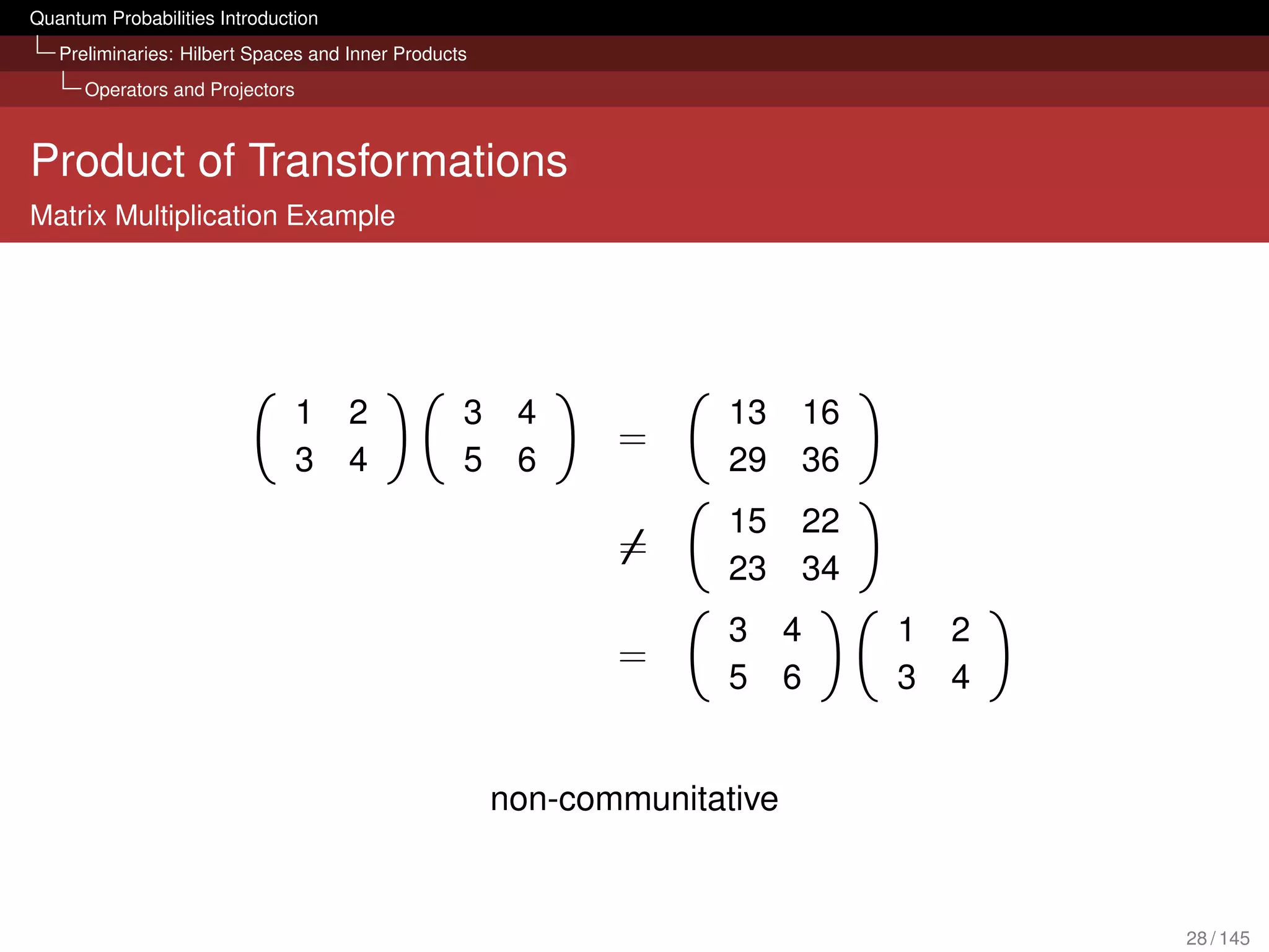
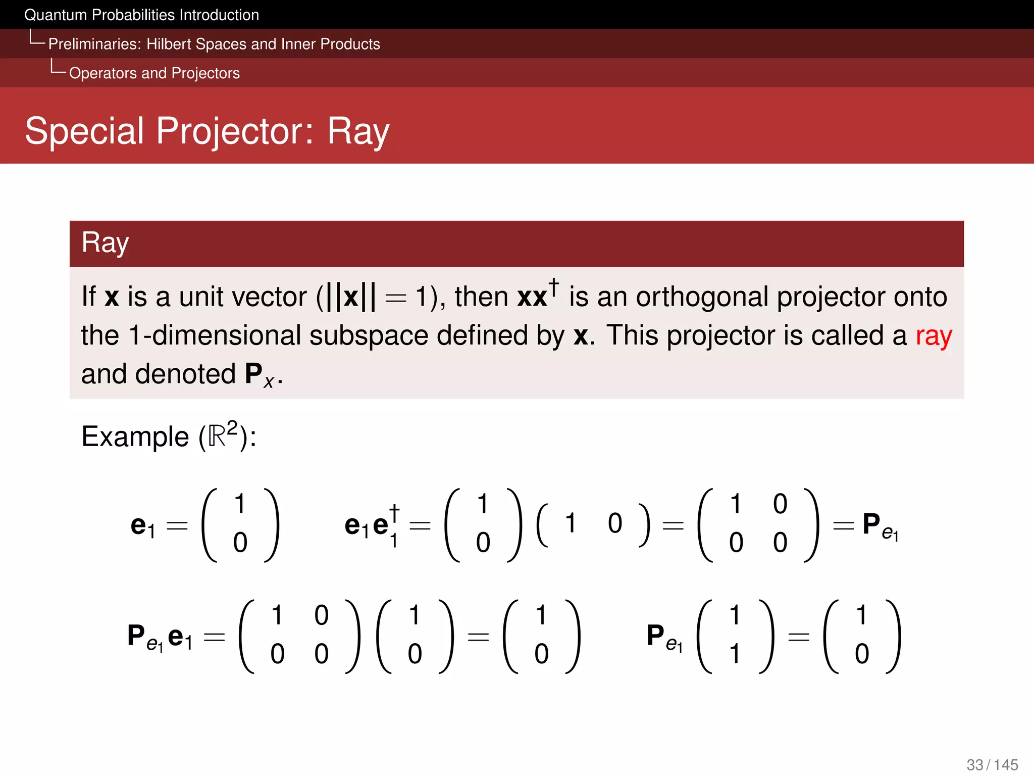
Operators and Projectors
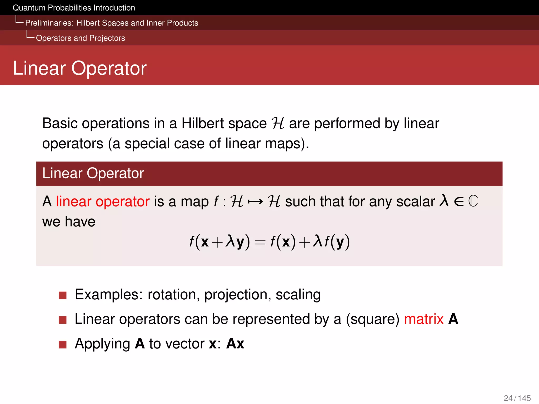
Towards Projectors
One of the most important operations for quantum probabilities
are projectors
We need to learn about linear operators and their matrix
representation first (see also [van Rijsbergen, 2004, Chapter 4])
23 / 145

24. Quantum Probabilities Introduction
Preliminaries: Hilbert Spaces and Inner Products
Operators and Projectors
Linear Operator
Basic operations in a Hilbert space H are performed by linear
operators (a special case of linear maps).
Linear Operator
A linear operator is a map f : H → H such that for any scalar λ ∈ C
we have
f (x + λy) = f (x) + λf (y)
Examples: rotation, projection, scaling
Linear operators can be represented by a (square) matrix A
Applying A to vector x: Ax
24 / 145

25. Quantum Probabilities Introduction
Preliminaries: Hilbert Spaces and Inner Products
Operators and Projectors
Operators as Matrices
n
yi = aik xk
k =1
25 / 145

26. Quantum Probabilities Introduction
Preliminaries: Hilbert Spaces and Inner Products
Operators and Projectors
Product of Transformations
Commutativity
The product of two transformations A and B is defined by the
effect it has on the vector x
ABx means: Apply B to x then apply the result to A
ABx is usually (but not always) different from BAx
If ABx = BAx, that is AB = BA, A and B are said to be
commutative (commuting)
They are non-commutative if AB = BA
26 / 145

27. Quantum Probabilities Introduction
Preliminaries: Hilbert Spaces and Inner Products
Operators and Projectors
Product of Transformations
Matrix Multiplication
AB = C
n
cij = aik bkj
k =1
27 / 145

28. Quantum Probabilities Introduction
Preliminaries: Hilbert Spaces and Inner Products
Operators and Projectors
Product of Transformations
Matrix Multiplication Example
1 2 3 4 13 16
=
3 4 5 6 29 36
15 22
=
23 34
3 4 1 2
=
5 6 3 4
non-communitative
28 / 145

29. Quantum Probabilities Introduction
Preliminaries: Hilbert Spaces and Inner Products
Operators and Projectors
Adjoints
Adjoint and Self-Adjoint (Hermitian)
The adjoint of a linear operator (or matrix) A is an operator A† so that
〈A† x, y〉 = 〈x, Ay〉
An operator/matrix is self-adjoint (Hermitian) if A = A† .
When the scalars are complex: A† = AT (conjugate transpose)
In the real case: A† = AT symmetric (AT = A) and self-adjoint
matrices are the same
29 / 145

30. Quantum Probabilities Introduction
Preliminaries: Hilbert Spaces and Inner Products
Operators and Projectors
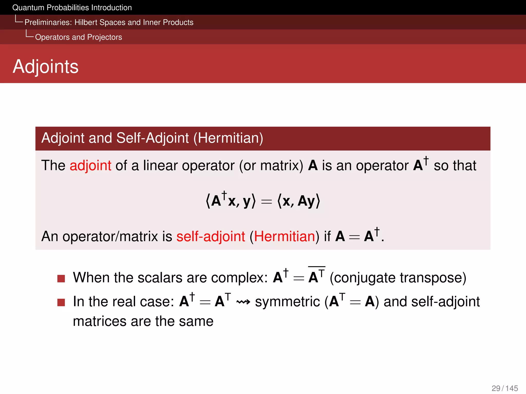
Adjoints
Example
Real case:
†
a x a u
=
u c x c
Complex case:
†
a + ib x − iy a − ib u + iv
=
u − iv c + id x + iy c − id
[van Rijsbergen, 2004, p. 55]
30 / 145

31. Quantum Probabilities Introduction
Preliminaries: Hilbert Spaces and Inner Products
Operators and Projectors
Orthogonal Projector
Orthogonal Projector
An orthogonal projector P is an idempotent, self-adjoint linear operator
in H.
Idempotent: P = PP (P leaves its image unchanged)
There is a one-to-one correspondence between orthogonal
projectors and subspaces
Each vector orthogonal to the subspace projects to 0
We use the notation P to denote the orthogonal projector (a
matrix) that represents a subspace
31 / 145

32. Quantum Probabilities Introduction
Preliminaries: Hilbert Spaces and Inner Products
Operators and Projectors
Orthogonal Projector
Example
 
1 0 0
P= 0 1 0 
 
0 0 0
z  
x 0
z =  0  orthogonal to P,
 
Px y = Py 1
hence Pz = 0
P
 
0
y =  1  contained in P,
 
0
so projection has no effect
32 / 145

33. Quantum Probabilities Introduction
Preliminaries: Hilbert Spaces and Inner Products
Operators and Projectors
Special Projector: Ray
Ray
If x is a unit vector (||x|| = 1), then xx† is an orthogonal projector onto
the 1-dimensional subspace defined by x. This projector is called a ray
and denoted Px .
Example (R2 ):
1 † 1 1 0
e1 = e1 e1 = 1 0 = = Pe1
0 0 0 0
1 0 1 1 1 1
Pe1 e1 = = Pe1 =
0 0 0 0 1 0
33 / 145

34. Quantum Probabilities Introduction
Preliminaries: Hilbert Spaces and Inner Products
Operators and Projectors
Spectral Theorem
Spectral Theorem
To any self-adjoint matrix A on a finite-dimensional complex inner
product space V there correspond real numbers α1 , . . . , αr and
projectors E1 , . . . , Er , r ≤ dim(V), so that
1 the αj are pairwise distinct;
2 the Ej are mutually orthogonal;
r
3 E = I (I is
j =1 j
the identity matrix);
r
4 A = j =1 αj Ej
Orthogonality: Ei ⊥Ej iff Ei Ej = Ei Ej = 0
The αj are the distinct eigenvalues of A
The Ej are the subspaces generated by the eigenvectors
34 / 145

35. Quantum Probabilities Introduction
Preliminaries: Hilbert Spaces and Inner Products
Operators and Projectors
Spectral Theorem
Simple Example
 
1 0 0
A= 0 0 0  Eigenvalues α1 = 1 α2 = 0
 
0 0 0
   
1 0 0 0 0 0
A = α1  0 0 0  +α2  0 1 0 
   
0 0 0 0 0 1
E1 E2
 
1
†
Eigenvector e1 =  0 : e1 e1 = E1
 
0
35 / 145

36. Quantum Probabilities Introduction
Preliminaries: Hilbert Spaces and Inner Products
Tensor Spaces
Tensor Space
A number of Hilbert spaces H1 , . . . , Hn can be combined to a
composite tensor space H = H1 ⊗ . . . ⊗ Hn
If eij is an orthonormal basis of Hi , then
eij
i ,j
(the tensor product of all combination of basis vectors) is an
orthonormal basis of the tensor space
36 / 145

37. Quantum Probabilities Introduction
Preliminaries: Hilbert Spaces and Inner Products
Tensor Spaces
Tensor Space
Example
C2 ⊗ C2 is a 4-dimensional space C4 with base vectors
1 2
e1 ⊗ e2 , e1 ⊗ e2 , e1 ⊗ e2 , e1 ⊗ e2
1 1 1 2 2 1 2 2
( e1 and e2 base vectors of C2 and C2 , respectively)
i j 1 2
37 / 145

38. Quantum Probabilities Introduction
Preliminaries: Hilbert Spaces and Inner Products
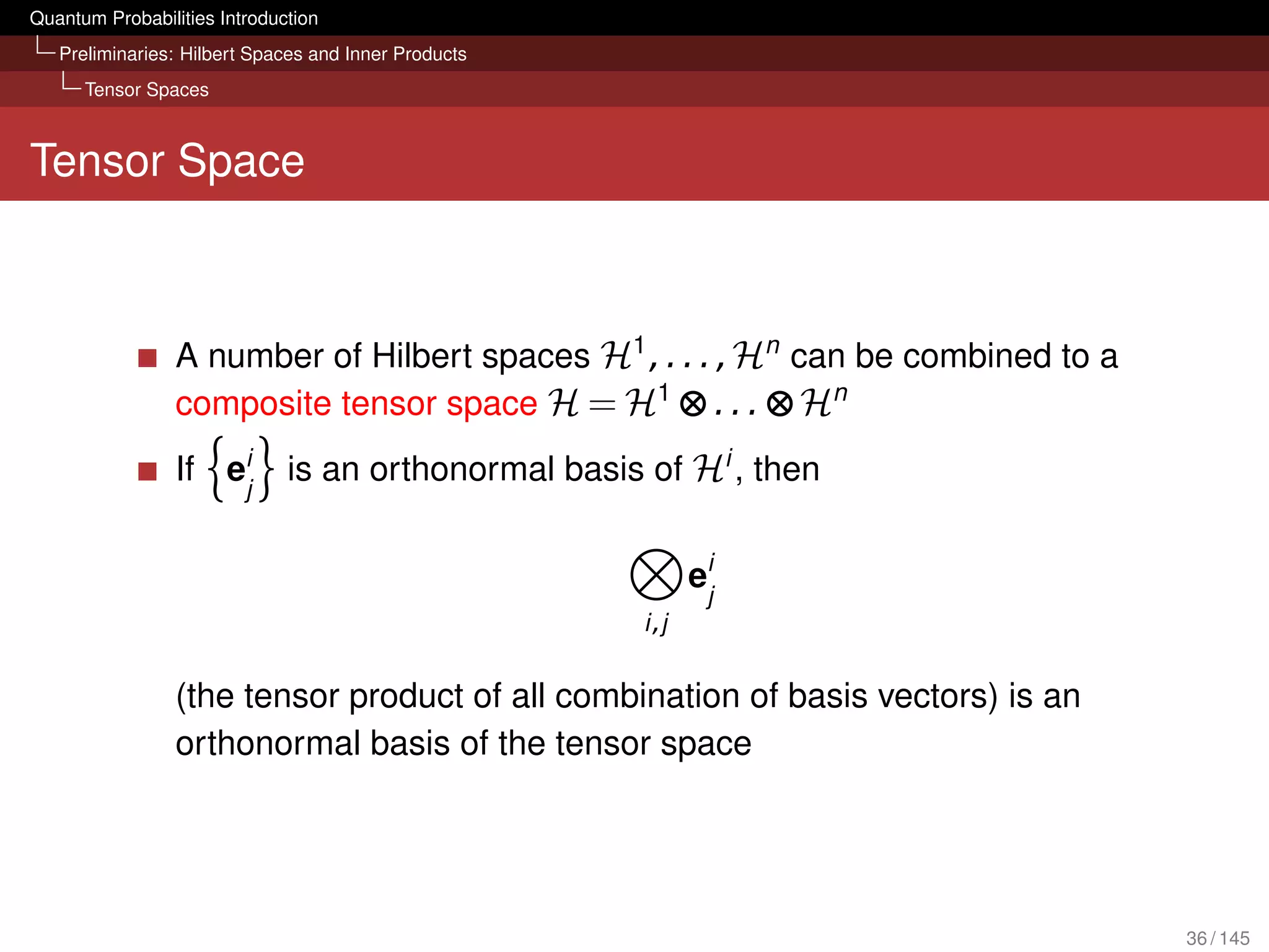
Tensor Spaces
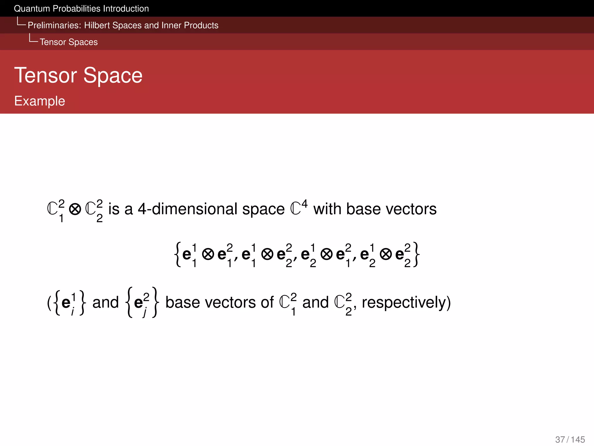
Tensor Space
Product Operators
If A is an operator in H1 and B is an operator in H2 , then A ⊗ B is
an operator in H1 ⊗ H2 and it is
(A ⊗ B)(a ⊗ b) = Aa ⊗ Bb
for a ∈ H1 , b ∈ H2 and a ⊗ b ∈ H1 ⊗ H2 .
A matrix representation for the tensor product is given by the
Kronecker product (see also [Nielsen and Chuang, 2000, p. 74])
38 / 145

39. Quantum Probabilities Introduction
Quantum Probabilities
Quantum Probabilities
39 / 145

40. Quantum Probabilities Introduction
Quantum Probabilities
Quantum Probabilities
40 / 145

41. Quantum Probabilities Introduction
Quantum Probabilities
Quantum and Classical Probabilities
Quantum and Classical Probabilities
Quantum probabilities are used in quantum theory to describe the
behaviour of matter at atomic and subatomic scales
Quantum probabilities are a generalisation of classical probability
theory
41 / 145

42. Quantum Probabilities Introduction
Quantum Probabilities
Quantum and Classical Probabilities
Quantum and Classical Probabilities
Correspondance
Sample space Set Hilbert space
Atomic event Element Ray
Event Subset Subspace
Null element Empty set Empty space
Membership Indicator function Projector
Exclusiveness Empty intersection Empty intersection
42 / 145

43. Quantum Probabilities Introduction
Quantum Probabilities
Dirac Notation
Dirac Notation
In many textbooks on quantum mechanics a different (and quite
handy) notation is used for vectors, the so-called Dirac notation
(named after Paul Dirac).
Dirac Notation
A vector y in a Hilbert space H is represented by a |y 〉, a ket. A bra
〈x | denotes a linear functional (a map f : H → K). Thus the bra(c)ket
〈x |y 〉 denotes the inner product 〈x, y〉 = x† y = f (y).
〈x | = (|x 〉)† (adjoint) if K = C
〈x | = (|x 〉)T (transpose) if K = R
Bra linear: 〈x | (α |y 〉 + β |z 〉) = α〈x |y 〉 + β〈x |z 〉
43 / 145

44. Quantum Probabilities Introduction
Quantum Probabilities
Dirac Notation
Dyads
Dyads are a special class of operators
Outer product of a ket and a bra (a matrix!): |x 〉〈y |
In particular useful to describe (projectors onto) rays: Px = |x 〉〈x |
Example:
0 0 0
0 1 =
1 0 1
44 / 145

45. Quantum Probabilities Introduction
Quantum Probabilities
Dirac Notation
Notation
Vector x or |x 〉
Adjoint x† or 〈x | or A† (for matrices)
Inner product 〈x, y〉 or x† y or 〈x |y 〉
Projector S projects onto subspace S (and represents it)
Ray Px ray projector determined by |x 〉
Standard probability Pr
Quantum probability Pr
45 / 145

46. Quantum Probabilities Introduction
Quantum Probabilities
Events
Events
An event S in quantum probabilities is described by the subspace
S
Atomic events are 1-dimensional subspaces (rays)
Combination of events (a glimpse into quantum logics):
Join ∨: spanning subspace
Meet ∧: biggest included subspace
Complement ⊥ : orthogonal subspace
If S1 and S2 commute:
S1 ∨ S2 = S1 + S2 − S1 S2
S1 ∧ S2 = S1 S2
S⊥ = I − S (I identity matrix)
46 / 145

47. Quantum Probabilities Introduction
Quantum Probabilities
Quantum Logics
Quantum Logic
Violation of distributive law
Let
1 1/ 2 0
|φ1 〉 = |φ2 〉 = |φ3 〉 =
0 1/ 2 1
Then
|φ1 〉
(Pφ1 ∧ Pφ2 ) ∨ Pφ3 = Pφ3 |φ2 〉
Pφ3 |φ3 〉
but
(Pφ1 ∨ Pφ3 ) ∧ (Pφ2 ∨ Pφ3 ) = I
Pφ2
Pφ1
47 / 145

48. Quantum Probabilities Introduction
Quantum Probabilities
Quantum Logics
The Classical Case
Quantum logics and probability reduces to classical logic and
probability if all measures are compatible
Compatibility basically means that the involved projectors are
commuting (so the order does not matter)
This happens when all event rays are orthogonal
48 / 145

49. Quantum Probabilities Introduction
Quantum Probabilities
Quantum States
Quantum states
Quantum probabilities are induced by quantum states
A pure quantum state (or pure state) is represented by a unit
vector |φ〉 (the state vector) in the Hilbert space H
A mixed (quantum) state is a probabilistic mixture of pure states
Both kinds of states can be described by probability densities (a
matrix with trace 1)
49 / 145

50. Quantum Probabilities Introduction
Quantum Probabilities
Pure States
Quantum Probabilities: Pure state
Quantum probability (pure state)
The probability of the event S given the state φ is the squared length
of the projection onto the corresponding subspace S:
2
Pr(S |φ) = ||S |φ〉||
|φ〉
S |φ〉
S
50 / 145

51. Quantum Probabilities Introduction
Quantum Probabilities
Pure States
Vector Space Model
An example “quantum” system
We are now ready to build our first “quantum” IR system
Vector space model: document d and query q normalised vectors
|d 〉 and |q 〉 in term space Rn
|q 〉 state vector, Pd = |d 〉〈d |
|d 〉
2 2 |q 〉
Pr(d |q ) = ||Pd |q 〉|| = |||d 〉 〈d |q 〉||
= ||〈d , q 〉||2 = cos2 (θ)
= ||〈q , d 〉||2 = |||q 〉 〈q |d 〉||2
θ
2
= Pq | d 〉 =Pr(q |d )
|d 〉 state vector, Pq = |q 〉〈q | (dual view)
51 / 145

52. Quantum Probabilities Introduction
Quantum Probabilities
Pure States
Effect of Measurement
We have seen how we can express the probability of and event S
What happens if we observe or measure that an event occurs (for
instance the relevance of a document)?
The state needs to be updated
For a pure state φ this is just the normalised projection
|φ〉
S |φ〉
φ = |φ〉 S= S |φ〉
||S |φ〉||
S
An immediate observation of the same event would not change
the state any more (S |φ 〉 = |φ 〉, S idempotent!)
Pr(S |φ ) = 1
52 / 145

53. Quantum Probabilities Introduction
Quantum Probabilities
Pure States
Effect of Measurement
We have seen how we can express the probability of and event S
What happens if we observe or measure that an event occurs (for
instance the relevance of a document)?
The state needs to be updated
For a pure state φ this is just the normalised projection
S |φ〉
φ = |φ〉 S= |φ 〉
||S |φ〉||
S
An immediate observation of the same event would not change
the state any more (S |φ 〉 = |φ 〉, S idempotent!)
Pr(S |φ ) = 1
53 / 145

54. Quantum Probabilities Introduction
Quantum Probabilities
Pure States
Order Effects
Quantum probabilities provide a theory
|a〉
for explaining order effects
|b 〉
|x 〉
Such effects appear when incompatible
measures are involved
We sketch this with a simple example
X
B
A
54 / 145

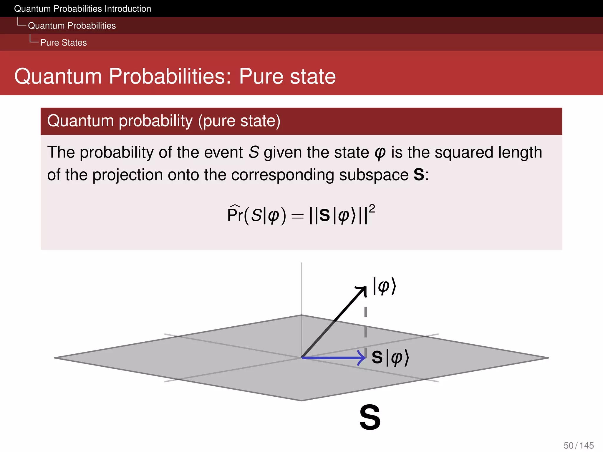
55. Quantum Probabilities Introduction
Quantum Probabilities
Pure States
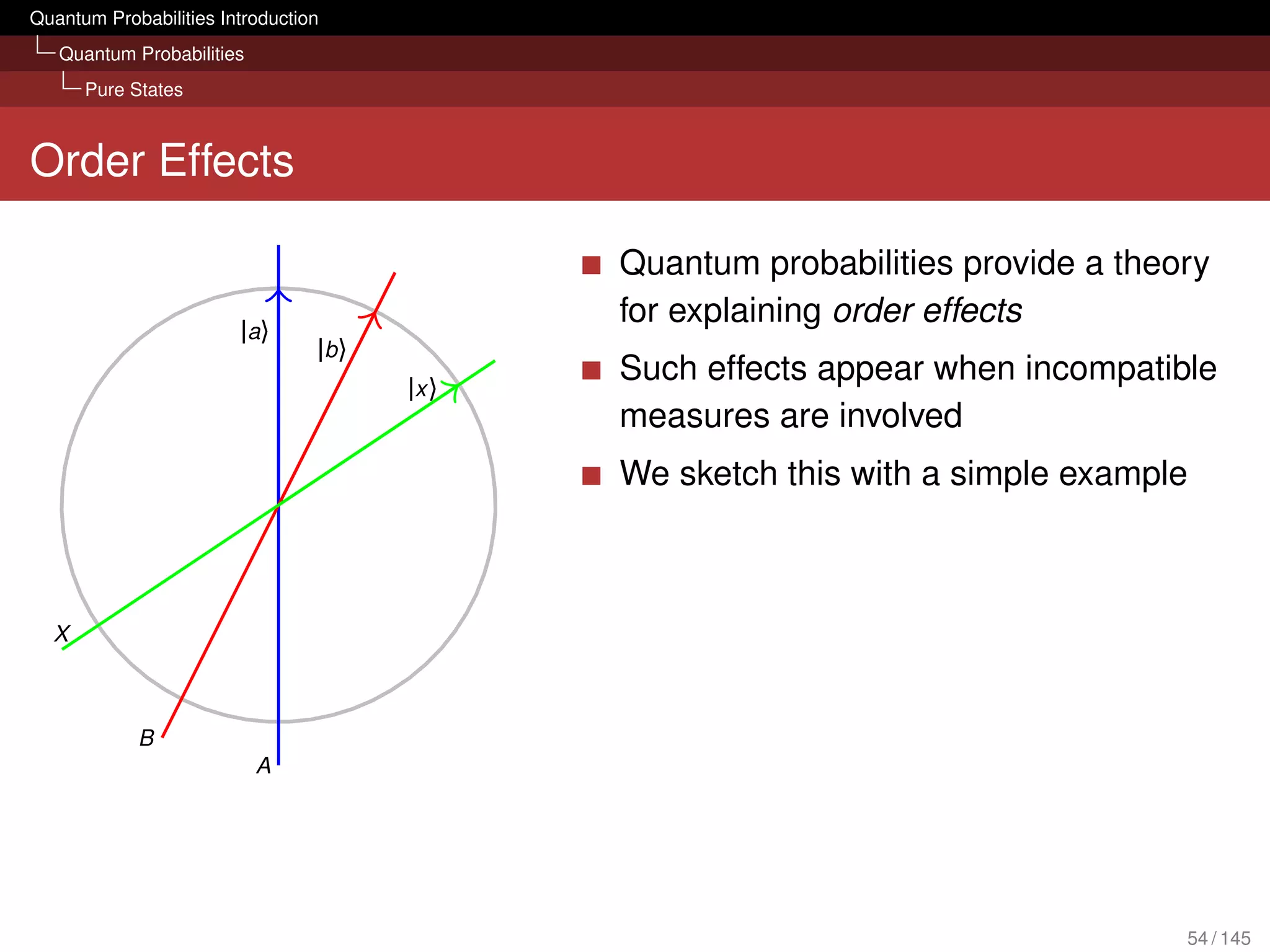
Order Effects
3 Events A,B,X
A = |a〉〈a|
|a〉
|b 〉 B = |b 〉〈b |
|x 〉
X = |x 〉〈x |
All non-commutative!
Pr(X |AB ) = Pr(X |BA)
The probability that we observe X is
different if we observed A then B or if we
X
observed B then A
[van Rijsbergen, 2004]: Determining
B relevance then aboutness is not the
A
same as determining aboutness then
relevance
55 / 145

56. Quantum Probabilities Introduction
Quantum Probabilities
Pure States
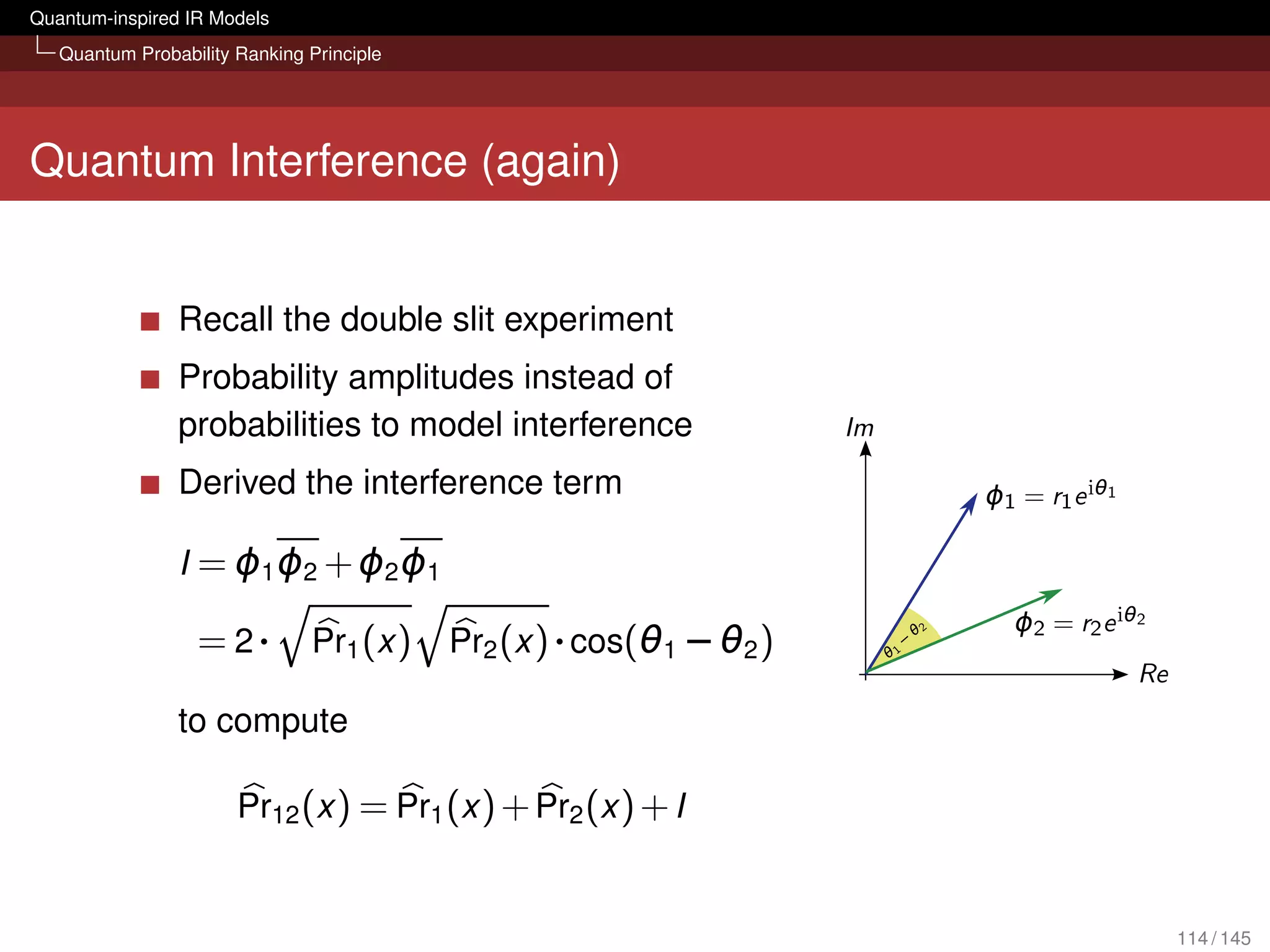
Interference
The Double Slit Experiment
(Taken from [Feynman, 1951])
Physical experiment that
motivates interference
Some works (e.g.
[Zuccon et al., 2009,
Melucci, 2010b]) use this
analogy for IR
Particle either passes slit 1 or
slit 2 before it appears
somewhere on the screen
Probability Pr(x ) that it
appears at position x?
56 / 145

57. Quantum Probabilities Introduction
Quantum Probabilities
Pure States
Interference
The Double Slit Experiment
(Taken from [Feynman, 1951])
Classical Kolmogorovian
probabilities:
Pr12 (x ) = Pr(x |slit 1 or slit 2)
= Pr(x |slit 1) + Pr(x |slit 2)
= Pr1 (x ) + Pr2 (x )
But this is not what we observe!
57 / 145

58. Quantum Probabilities Introduction
Quantum Probabilities
Pure States
Interference
The Double Slit Experiment
(Taken from [Feynman, 1951])
Quantum Probabilities: Use
probability amplitudes!
An amplitude ϕ is a complex
number
Refer to qubit example: ϕ
could be an inner product
Pr(x ) = |ϕ(x )|2
ϕ12 = ϕ(x |slit 1 or slit 2)
= ϕ(x |slit 1) + ϕ(x |slit 2)
= ϕ1 + ϕ2
58 / 145

59. Quantum Probabilities Introduction
Quantum Probabilities
Pure States
Interference
The Double Slit Experiment
(Taken from [Feynman, 1951])
Following [Zuccon, 2012, p. 80]
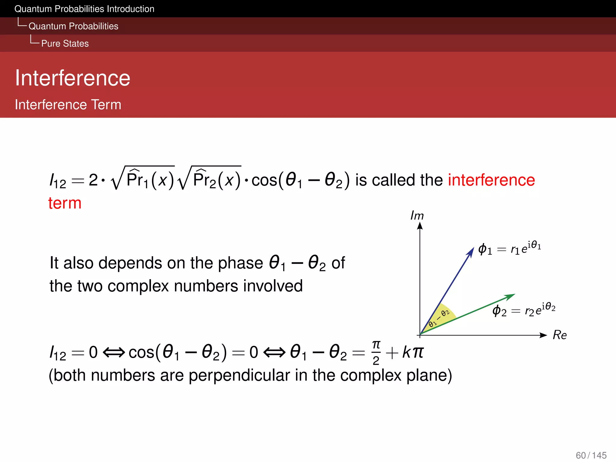
Pr12 (x ) = |ϕ12 |2 = |ϕ1 + ϕ2 |2
= |ϕ1 |2 + |ϕ2 |2 +
ϕ1 ϕ2 + ϕ2 ϕ1
= Pr1 (x ) + Pr2 (x )+
2· Pr1 (x ) Pr2 (x )·
cos(θ1 − θ2 )
= Pr1 (x ) + Pr2 (x ) + I12
with ϕ1 = r1 eiθ1 and ϕ2 = r2 eiθ2
59 / 145

60. Quantum Probabilities Introduction
Quantum Probabilities
Pure States
Interference
Interference Term
I12 = 2 · Pr1 (x ) Pr2 (x ) · cos(θ1 − θ2 ) is called the interference
term
It also depends on the phase θ1 − θ2 of
the two complex numbers involved
π
I12 = 0 ⇔ cos(θ1 − θ2 ) = 0 ⇔ θ1 − θ2 = 2 + k π
(both numbers are perpendicular in the complex plane)
60 / 145

61. Quantum Probabilities Introduction
Quantum Probabilities
Pure States
Composite Systems
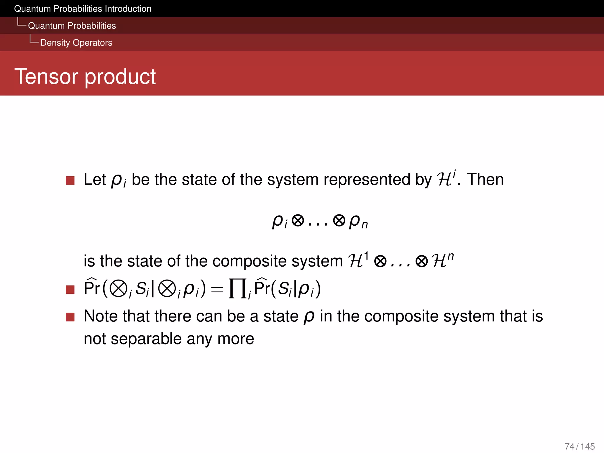
Tensor Spaces
Quantum systems (Hilbert spaces) can be combined using the
tensor product (see also [Griffiths, 2002])
If |φi 〉 ∈ Hi is the state of system i then
|φi 〉
i
is the state in the composite system i Hi (product state)
Let Si be a subspace (event) in Hi . Then
Pr Si | φi = Pr(Si |φi ) (1)
i i i
61 / 145

62. Quantum Probabilities Introduction
Quantum Probabilities
Pure States
Composite Systems
2 Qubit Example, Separable State
|1〉 |1〉 Combining two qubits with
|φ1 〉
|φ2 〉
|φ1 〉 = a1 |0〉 + a2 |1〉
|φ2 〉 = b1 |0〉 + b2 |1〉
|0〉 |0〉
State of composite system is the product state
|φ1 〉 ⊗ |φ2 〉 = a1 b1 |00〉 + a1 b2 |01〉 + a2 b1 |10〉 + a2 b2 |11〉
(with, e.g., |01〉 = |0〉 ⊗ |1〉)
If composite state is a product state, it is said to be separable
Both systems are independent – if we measure, say, |1〉in the first
qubit1 , we can still measure either |0〉 or |1〉 in the second one!
Bivariate distribution with ai , bi as marginals [Busemeyer, 2012]
1
Expressed by the subspace |10〉〈10| + |11〉〈11|
62 / 145

63. Quantum Probabilities Introduction
Quantum Probabilities
Pure States
Composite Systems
Entanglement
There are states in a composite system that cannot be expressed
as product states
For example in the 2 qubit system,
1 1
|φ〉 = |00〉 + |11〉
2 2
is such a non-separable state
The systems are not independent any more – if for instance we
measure |0〉 in the first qubit, this means the second qubit will be
in state |0〉!
The composite system is in an entangled state
Equation 1 does not hold any more
63 / 145

64. Quantum Probabilities Introduction
Quantum Probabilities
Mixed States
Mixed State
In general we don’t know the state of
the system (or in IR we don’t know |φ1 〉 (Pr(φ1 ))
|φ2 〉 (Pr(φ2 ))
what the user really wants) |φ3 〉 (Pr(φ3 ))
We assume the system to be in a S
certain state with a certain
(classical!) probability
Mixed (Quantum) State
We assume the system is in a state φi with probability Pr(φi ) so that
i Pr(φi ) = 1. Then the probability of an event S is
2
Pr(S ) = Pr(φi )Pr(S |φi ) = Pr(φi ) ||S |φi 〉||
i i
64 / 145

65. Quantum Probabilities Introduction
Quantum Probabilities
Mixed States
The Effect of Measurement
Mixed State
When observing/measuring S all state vectors are projected and
renormalised, resulting in a new state set {ψi }
The probability of each new state ψi is computed as follows:
Pr(S |φ) Pr(φ)
Pr(ψi |S ) =
φ|ψi =|φ〉 S
Pr(S )
φ|ψi = |φ〉 S means all vectors that have the same normalised
projection |ψi 〉
Conditional quantum probabilities:
Pr(S2 |S1 ) = Pr(S2 |ψ) Pr(ψ|S1 )
ψ
65 / 145

66. Quantum Probabilities Introduction
Quantum Probabilities
Density Operators
Preliminaries: Trace
Trace
n
tr(T) = 〈ei | T |ei 〉
i =1
is known as the trace of T with {|ei 〉} as an orthonormal basis. It is
equal to the sum of the diagonal elements of T.
Some important properties (see [van Rijsbergen, 2004, p. 79]):
Linearity: tr(α T1 + βT2 ) = α tr(T1 ) + βtr(T2 )
Cyclic permutation: e.g. tr(T1 T2 ) = tr(T2 T1 )
trT† = tr(T)
tr(T) ≥ 0 if T is positive definite
An operator T is of trace class if T is positive and its trace is finite
66 / 145

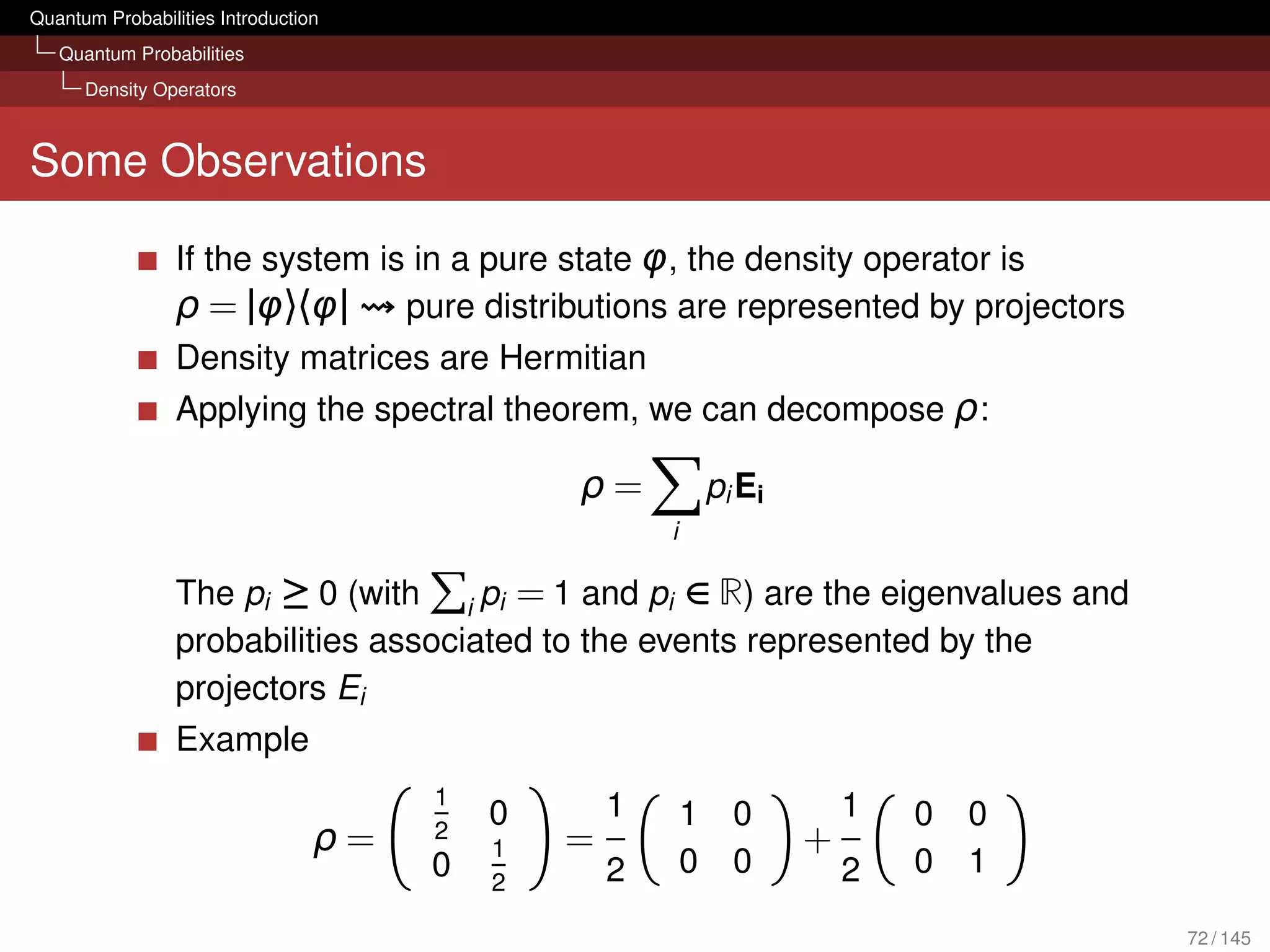
67. Quantum Probabilities Introduction
Quantum Probabilities
Density Operators
Trace and Probability
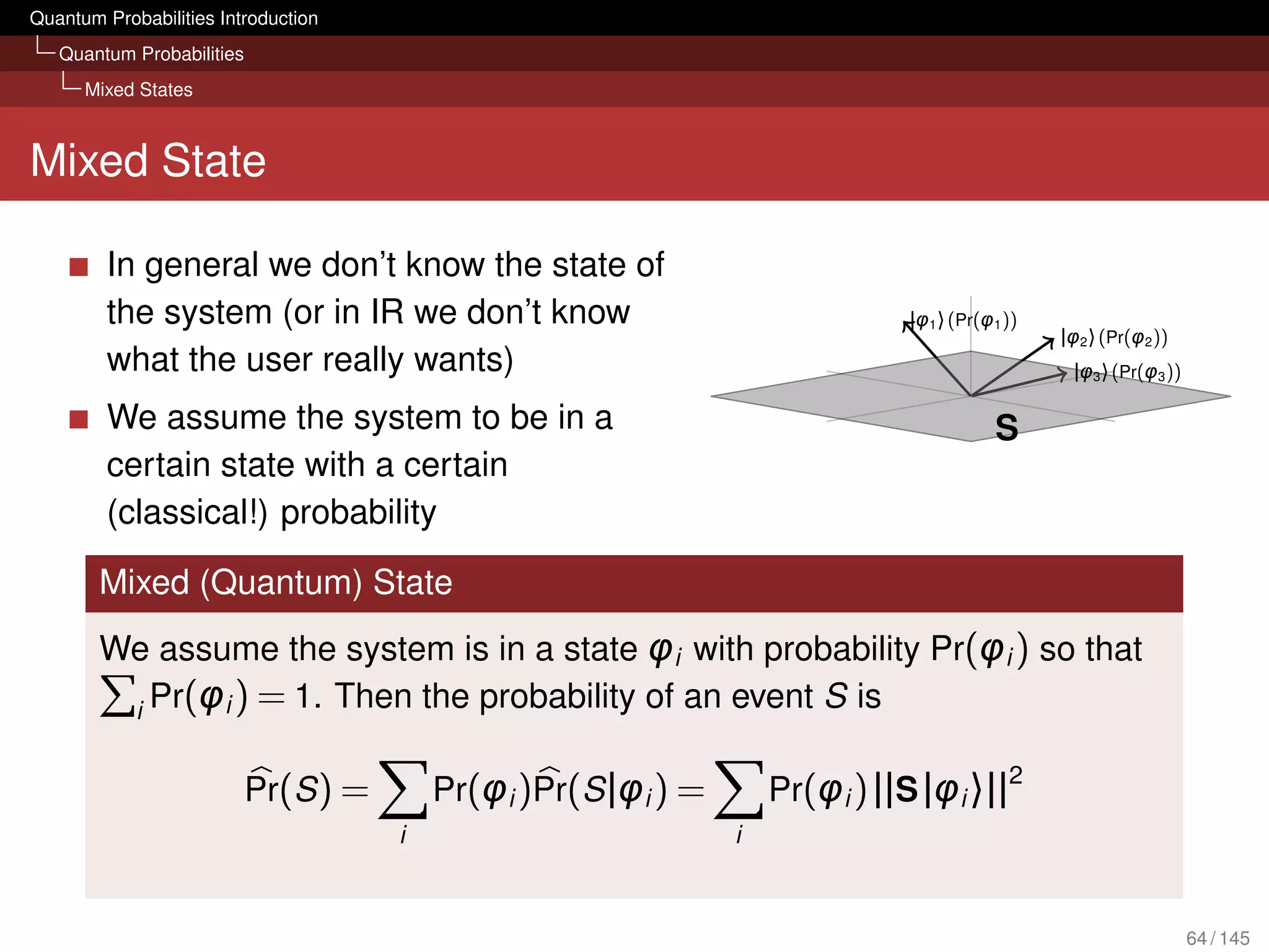
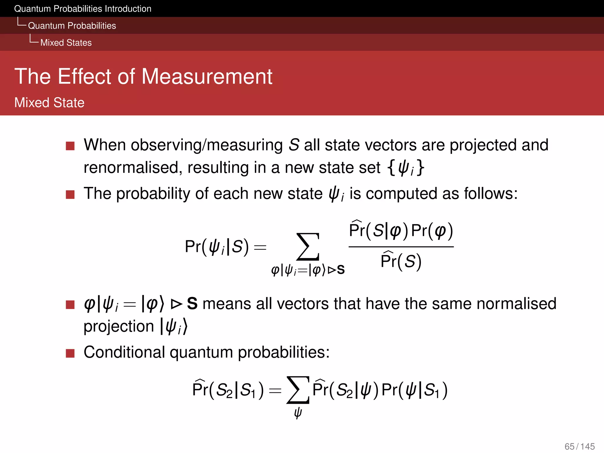
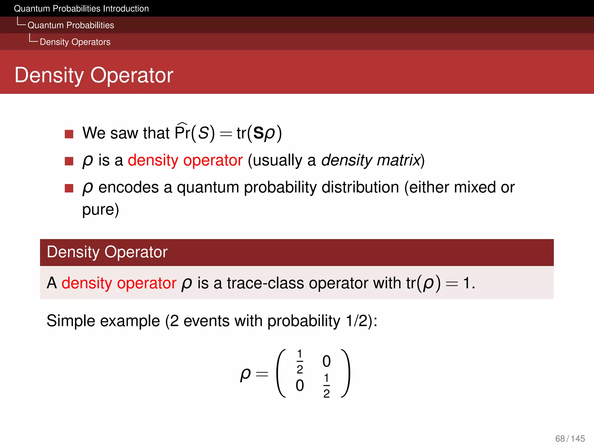
Density Operator
2
Pr(S ) = Pr(φi ) ||S |φi 〉||
i
= Pr(φi )〈Sφi |Sφi 〉 Def. norm
i
= Pr(φi ) 〈φi | S |φi 〉 S self-adjoint, idempotent
i
= Pr(φi ) tr(S |φi 〉〈φi |) [Nielsen and Chuang, 2000, p. 76]
i
 
 
 
= tr S
 Pr(φi ) |φi 〉〈φi |
 Trace linearity
 i 
=ρ 67 / 145

68. Quantum Probabilities Introduction
Quantum Probabilities
Density Operators
Density Operator
We saw that Pr(S ) = tr(Sρ)
ρ is a density operator (usually a density matrix)
ρ encodes a quantum probability distribution (either mixed or
pure)
Density Operator
A density operator ρ is a trace-class operator with tr(ρ) = 1.
Simple example (2 events with probability 1/2):
1
0
ρ= 2
1
0 2
68 / 145

69. Quantum Probabilities Introduction
Quantum Probabilities
Density Operators
Gleason’s Theorem
Gleason’s Theorem
Let μ be any measure on the closed subspaces of a separable (real or
complex) Hilbert space H of dimension of at least 3. There exists a
positive self-adjoint operator T of trace class such that, for all closed
subspaces S of H,
μ(S ) = tr(TS)
If μ is a probability measure, then tr(T) = 1, so T is a density
operator.
69 / 145

70. Quantum Probabilities Introduction
Quantum Probabilities
Density Operators
Gleason’s Theorem
In other words...
Following the Piwowarski/Melucci tutorial:
Distribution over a Hilbert Space
A distribution over a Hilbert space H is any function
Pr : S ⊆ H → [0, 1] such that:
Pr(∅) = 0 and Pr(Pφ ) ≥ 0 ∀φ ∈ H
i Pr(Pei ) = 1 for any basis {ei }
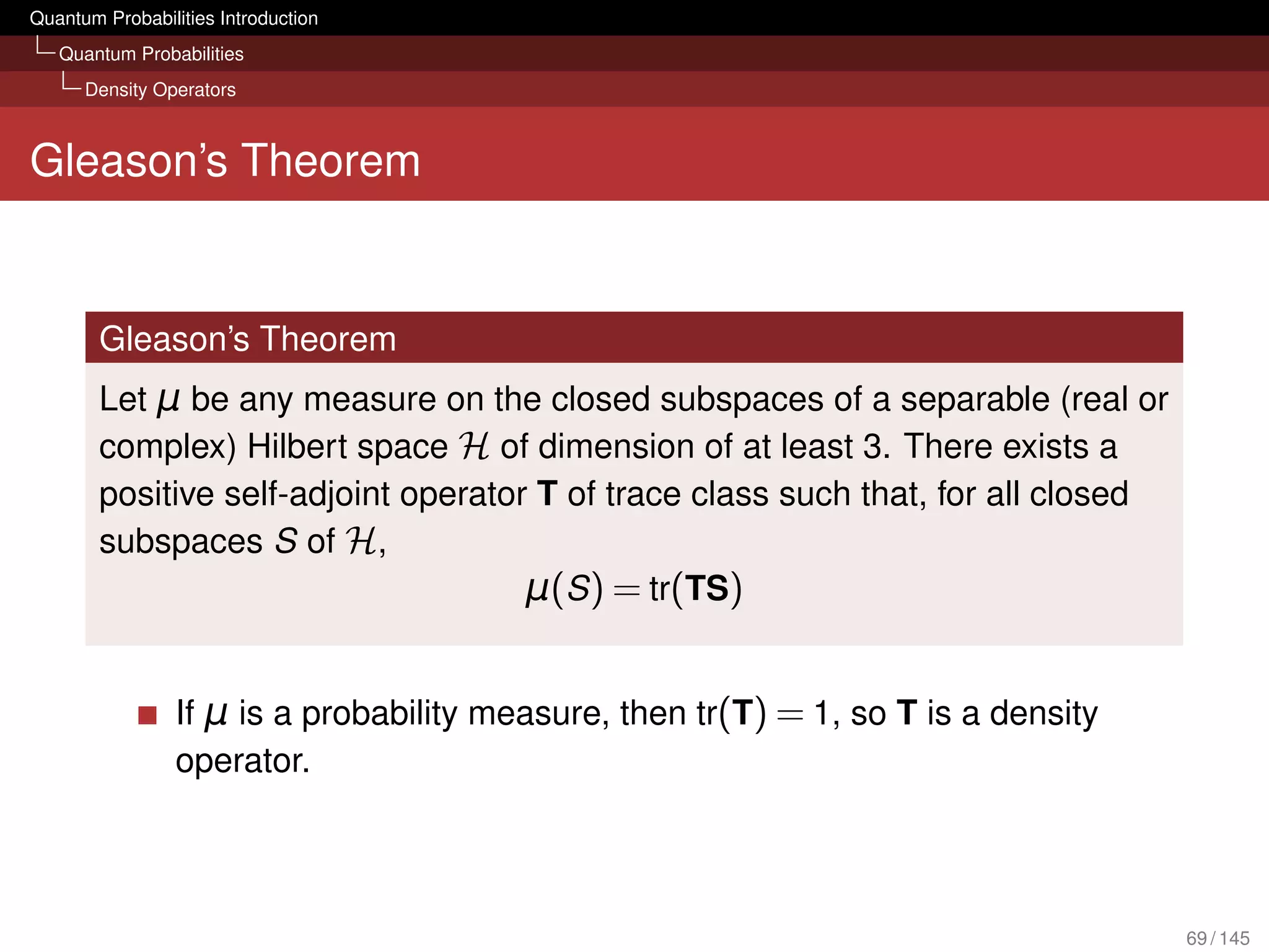
Gleason’s Theorem
To every probability distribution over a Hilbert space H (dimension
≥ 3), there exists a unique density matrix ρ such that for any S ⊆ H
Pr(S ) = tr(ρS)
70 / 145

71. Quantum Probabilities Introduction
Quantum Probabilities
Density Operators
What does this mean?
Gleason’s theorem provides a 1-to-1 relationship between
quantum probability distributions and density operators
We can approximate density operators using spectral techniques,
decompositions etc.
71 / 145

72. Quantum Probabilities Introduction
Quantum Probabilities
Density Operators
Some Observations
If the system is in a pure state φ, the density operator is
ρ = |φ〉〈φ| pure distributions are represented by projectors
Density matrices are Hermitian
Applying the spectral theorem, we can decompose ρ:
ρ= pi Ei
i
The pi ≥ 0 (with i pi = 1 and pi ∈ R) are the eigenvalues and
probabilities associated to the events represented by the
projectors Ei
Example
1 1 1
0 1 0 0 0
ρ= 2
1 = +
0 2 0 0 2 0 1
2
72 / 145

73. Quantum Probabilities Introduction
Quantum Probabilities
Density Operators
Measurement and Conditional Probabilities
Update of density matrix after measuring/observing S1 :
S1 ρ S1 S1 ρ S1
ρ = =
tr(S1 ρS1 ) tr(ρS1 )
Lüders’ Rule for conditional probabilities:
tr(S1 ρS1 S2 )
Pr(S2 |S1 ) =
tr(ρS1 )
If S1 and S2 are compatible, this reduces to classical
conditionalisation (see [Hughes, 1992, p. 224])
73 / 145

74. Quantum Probabilities Introduction
Quantum Probabilities
Density Operators
Tensor product
Let ρi be the state of the system represented by Hi . Then
ρi ⊗ . . . ⊗ ρn
is the state of the composite system H1 ⊗ . . . ⊗ Hn
Pr ( i Si | i ρi ) = i Pr(Si |ρi )
Note that there can be a state ρ in the composite system that is
not separable any more
74 / 145

75. Quantum Probabilities Introduction
Quantum Probabilities
Conclusion
Quantum Probabilities
Conclusion
Introduced quantum probabilities based on Hilbert Spaces
Some salient features: pure and mixed states, densities,
measurement/observation, order effects, interference, composite
systems, entanglement
Quantum probabilities as a generalisation of classical
probabilities
Now: How can we use this for information retrieval?
75 / 145

76. Quantum-inspired IR Models
The QIA Model
Quantum Information Access
Polyprepresentation
Quantum Probability Ranking Principle

77. Quantum Information Access (QIA)

78. Quantum-inspired IR Models
The QIA Model
Notation Wrap-Up
Hilbert space: vector space with an inner product
Dirac Notation:
|φ〉 is a ket (a vector φ)
〈φ| is a bra (a transposed vector φT )
〈φ|ψ〉 ∈ C is a bra(c)ket (inner product)
|φ〉〈ψ| is a ketbra (a matrix)
A subspace S is represented by a projector (another matrix)
|φ〉〈φ| projector onto 1-dimensional subspace
Orthogonal projection of vector |φ〉 onto S: S |φ〉
78 / 145

79. Quantum-inspired IR Models
The QIA Model
Quantum Information Access
Assumptions underlying QIA
IR system uncertain about user’s information need (IN)
System view of the user’s IN becomes more and more specific
through interaction
The IN may change from the user’s point of view
There is an IN Space, a Hilbert space
79 / 145

80. Quantum-inspired IR Models
The QIA Model
Quantum Information Access
Information Need Space
INs as vectors: IN
vector |φ〉
Event “document d is
relevant” represented
by subspace R
|quantum mechanics Probability of
relevance: squared
length of projection
Pr(R |d , φ) =
||R |φ〉 ||2
Unit vector imposes
relevance distribution
on subspaces (events)
80 / 145

81. Quantum-inspired IR Models
The QIA Model
Quantum Information Access
Information Need Space
INs as vectors: IN
vector |φ〉
Event “document d is
R relevant” represented
by subspace R
|quantum mechanics Probability of
relevance: squared
length of projection
Pr(R |d , φ) =
||R |φ〉 ||2
Unit vector imposes
relevance distribution
on subspaces (events)
81 / 145

82. Quantum-inspired IR Models
The QIA Model
Quantum Information Access
Information Need Space
INs as vectors: IN
vector |φ〉
Event “document d is
R relevant” represented
by subspace R
|quantum mechanics Probability of
relevance: squared
length of projection
Pr(R |d , φ) =
||R |φ〉 ||2
Unit vector imposes
relevance distribution
on subspaces (events)
82 / 145

83. Quantum-inspired IR Models
The QIA Model
Quantum Information Access
System’s Uncertainty about User’s Intentions
System uncertain about
user’s IN
p2
R Expressed by an ensemble S
p4
p5
of possible IN vectors (density
p1
ρ):
S = {(p1 , |φ1 〉) , . . . , (pn , |φn 〉)}
p3
Probability of relevance:
Pr(R |d , S ) = pi · Pr(R |d , φi )
i
=||R |φ〉||2
83 / 145

84. Quantum-inspired IR Models
The QIA Model
Quantum Information Access
System’s Uncertainty about User’s Intentions
p2
R
p4
p5 Dual representation using
p1
density operator and trace
function
ρ= i pi · |φi 〉〈φi |
Pr(R |d , S ) = tr(ρR )
p3
84 / 145

85. Quantum-inspired IR Models
The QIA Model
Quantum Information Access
User Interaction and Feedback
Outcome of feedback: Query
and query reformulation, (click
|ϕ2
on) relevant document, ...
R∗
|ϕ1 Expressed as subspace
|ϕ3
Project IN vectors onto
document subspace
Document now gets
probability 1
System’s uncertainty
|ϕ5
decreases
Also reflects changes in
information needs
85 / 145

86. Quantum-inspired IR Models
The QIA Model
Quantum Information Access
User Interaction and Feedback
Outcome of feedback: Query
and query reformulation, (click
|ϕ2
on) relevant document, ...
|ϕ4 R∗
|ϕ5 Expressed as subspace
Project IN vectors onto
|ϕ1
document subspace
Document now gets
probability 1
|ϕ3
System’s uncertainty
decreases
Also reflects changes in
information needs
86 / 145

87. Quantum-inspired IR Models
The QIA Model
Quantum Information Access
Textual Representation
IN Space / Documents
IN space based on term
space
IN vectors made of document
fragments
Weighting scheme (e.g., tf,
tf-idf,...)
Document is relevant to all
|jupiter crash
|jupiter (Term)
INs found in its fragments
Document subspace R
|crash (Term)
|car crash
spanned by IN vectors
No length normalisation
|car (Term)
necessary
|ϕ
87 / 145

88. Quantum-inspired IR Models
The QIA Model
Quantum Information Access
Single Query Term
Take all fragments vectors (IN
vectors) containing term t
This makes up ensemble St
88 / 145

89. Quantum-inspired IR Models
The QIA Model
Quantum Information Access
Mixture
Mixture of all combinations of
term fragments
Document must at least
satisfy one term fragment
The more term fragments are
contained, the more relevant
a document is
n
S (M ) = wS
i =1 i ti
wi is term weight
89 / 145

90. Quantum-inspired IR Models
The QIA Model
Quantum Information Access
Mixture of Superposition
Superpose all combinations
1
(e.g.
2
(|φ〉 + |ψ〉))
At least one query term
fragment superposition must
be contained
The more fragment
superpositions are contained,
the more relevant a document
is
Indication that it works well
with multi-term concepts (e.g.
“digital libraries”)
90 / 145

91. Quantum-inspired IR Models
The QIA Model
Quantum Information Access
Tensor product
Assumption: each term
covers an IN aspect
Tensor product of all fragment
vectors combination of IN
aspects
Document must satisfy all IN
aspects
The more tensor products are
satisfied, the more relevant is
the document
91 / 145

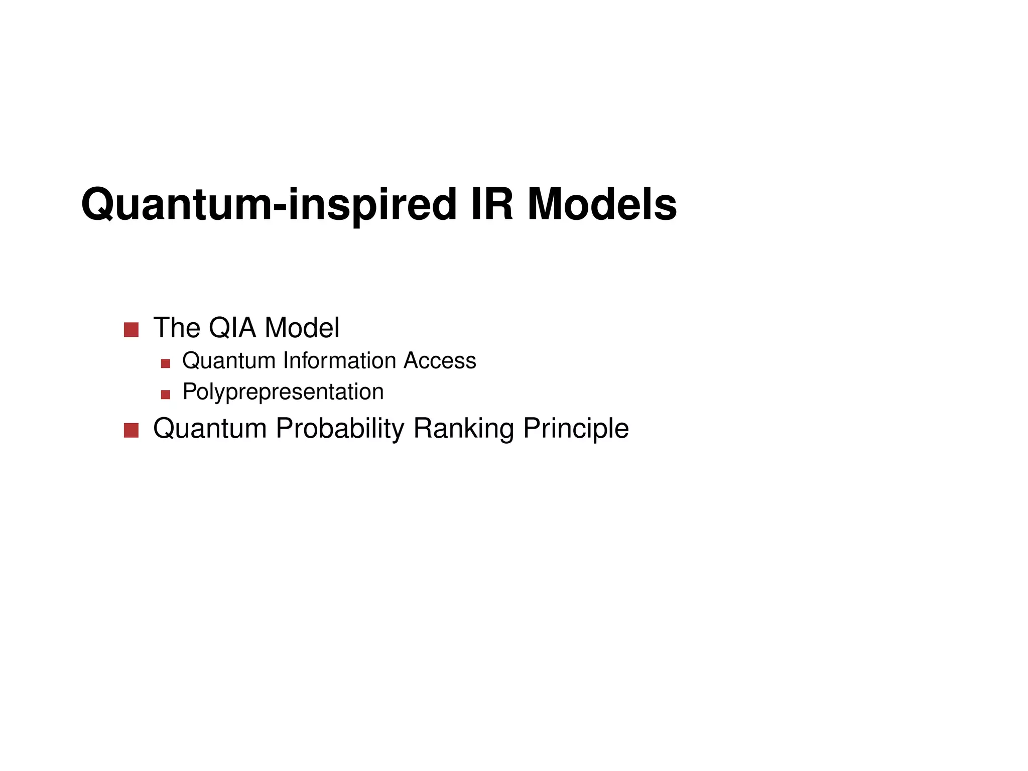
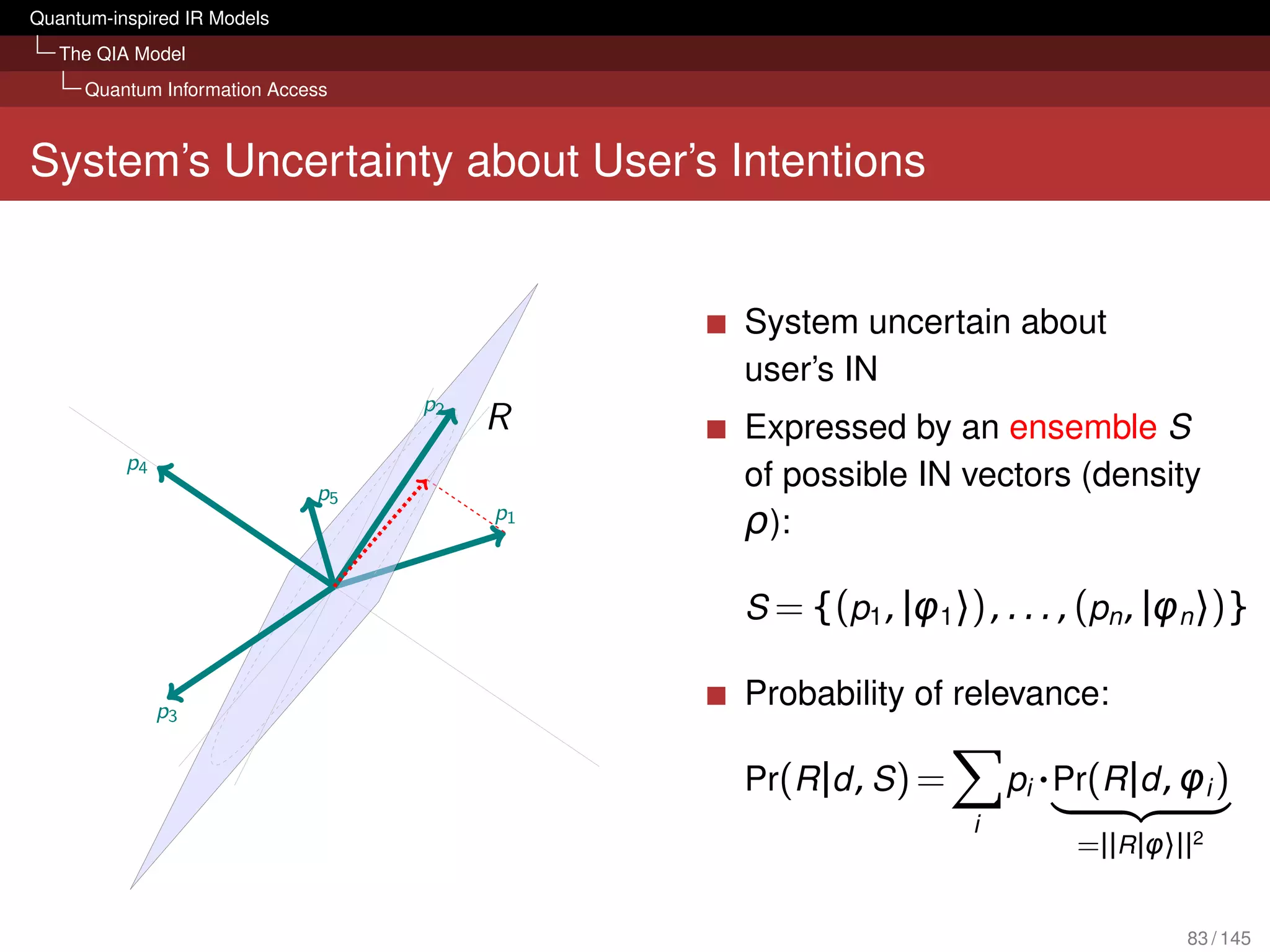
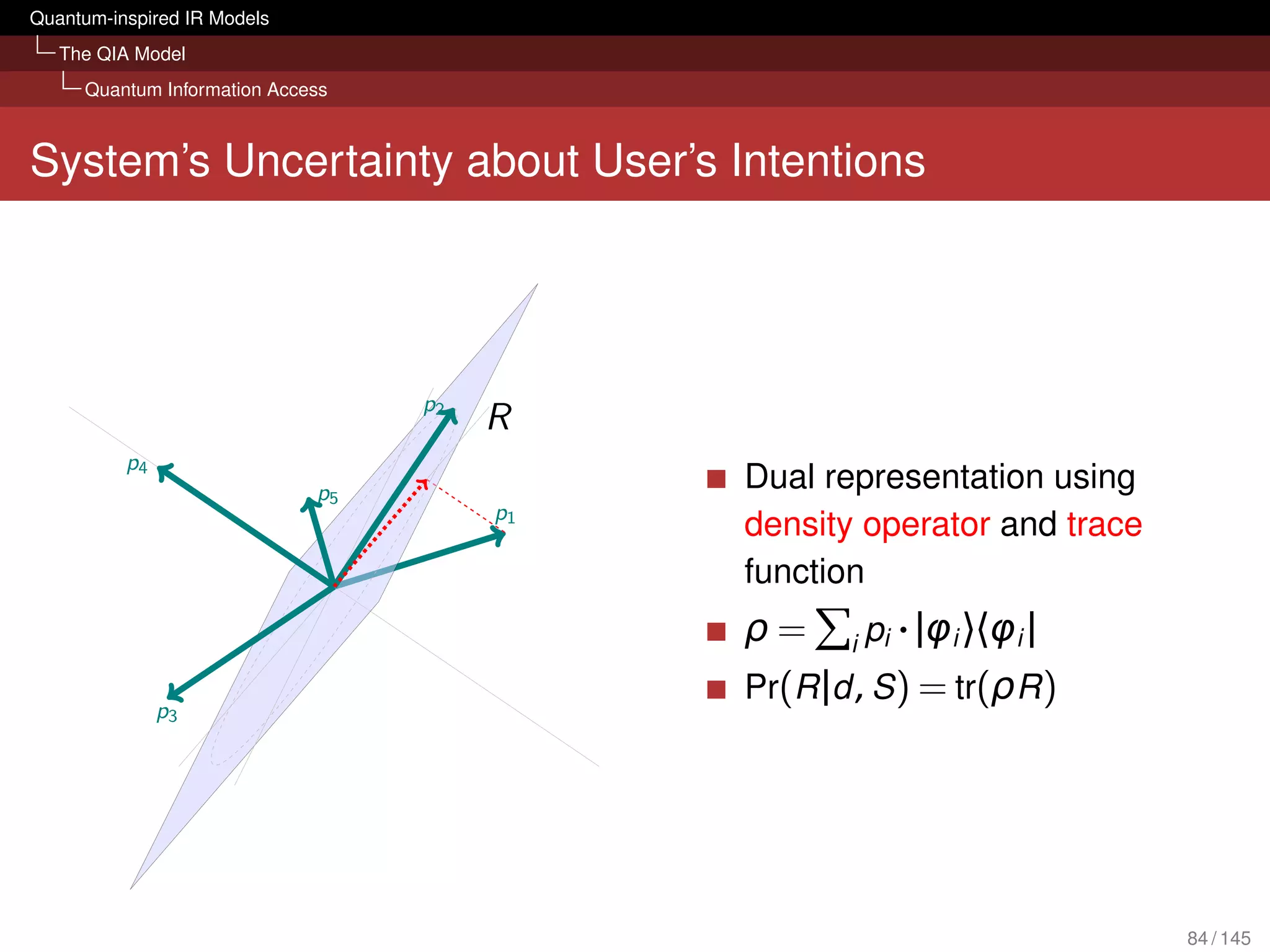
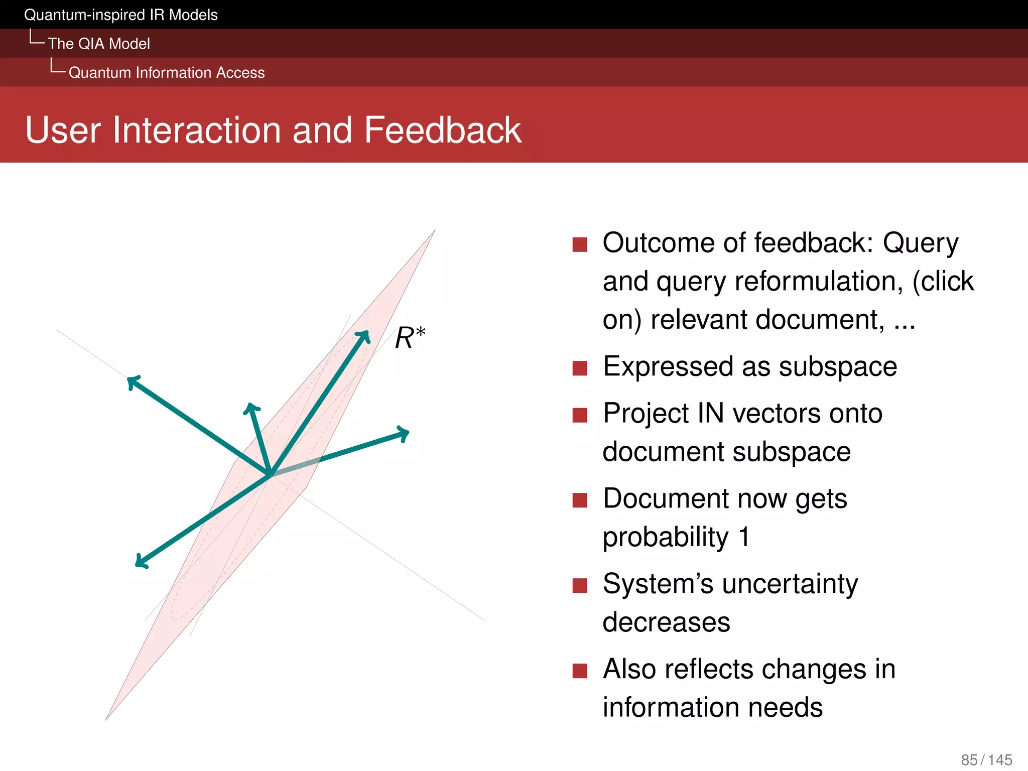
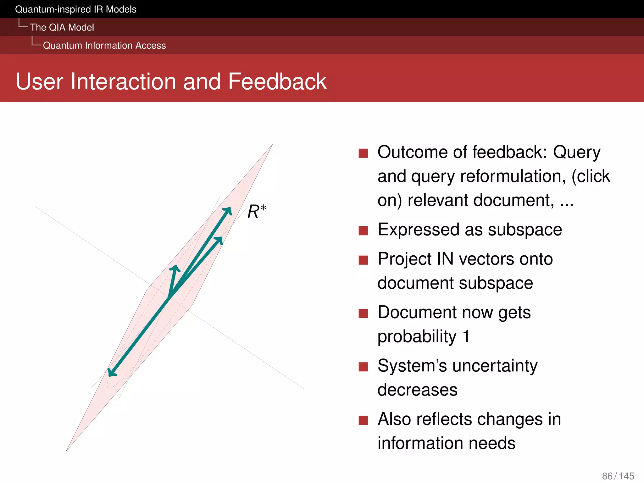
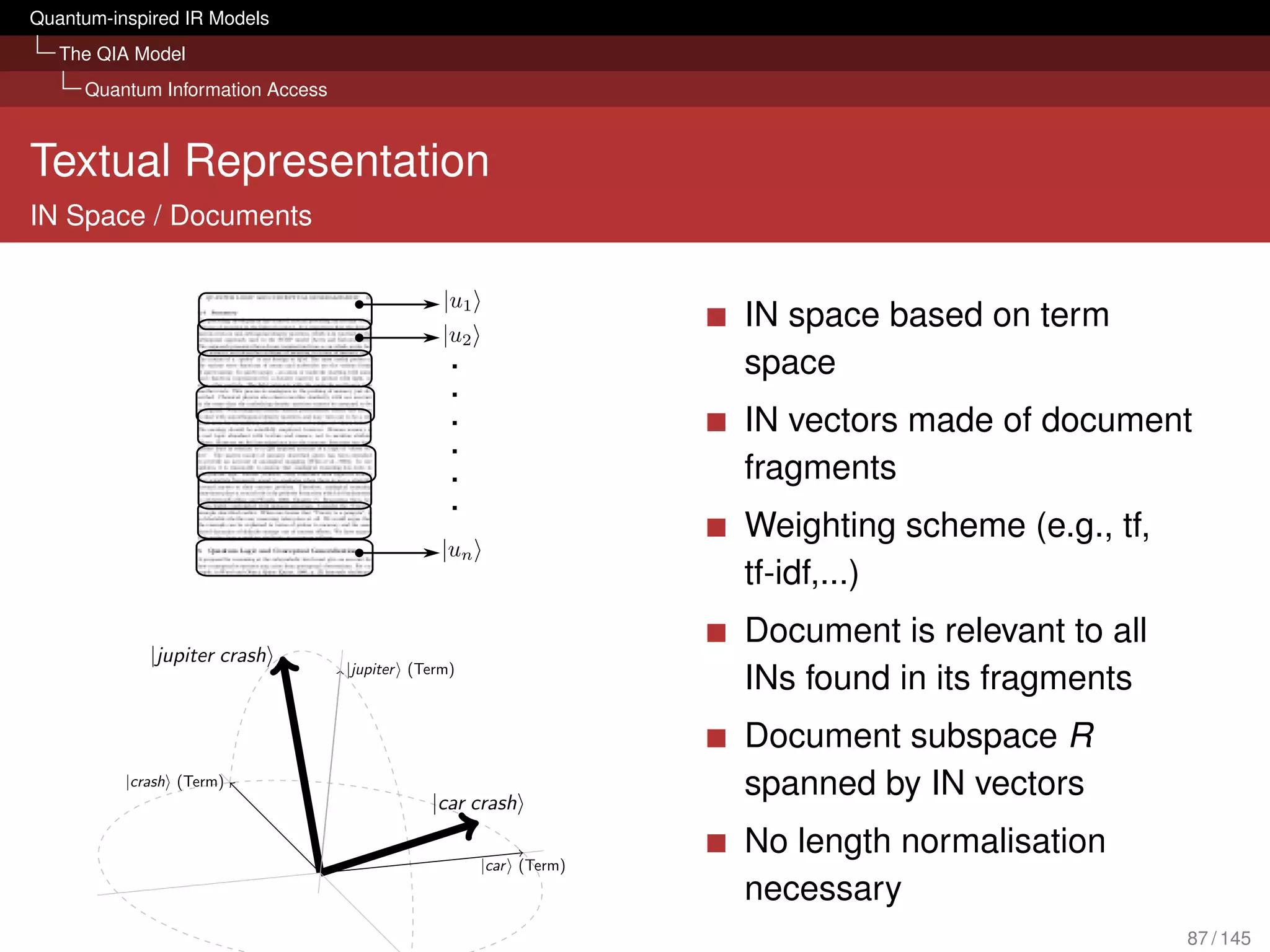
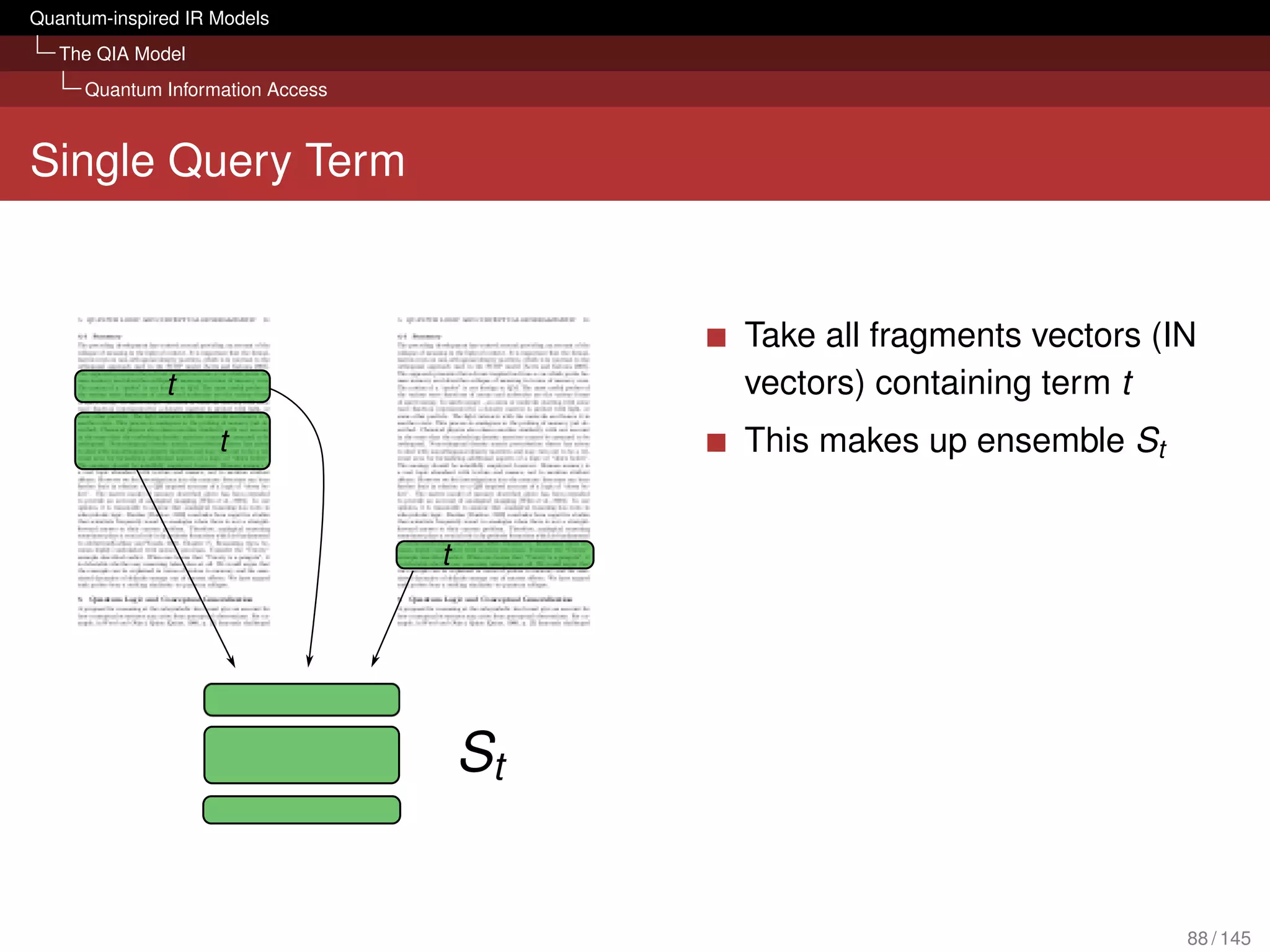
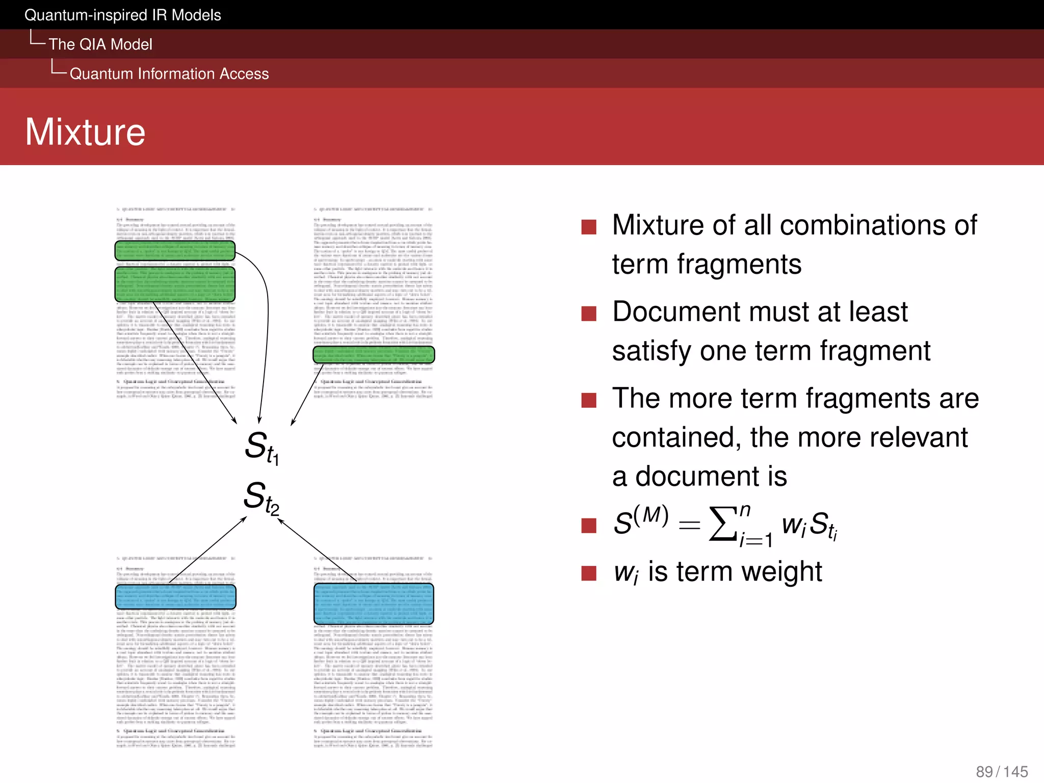
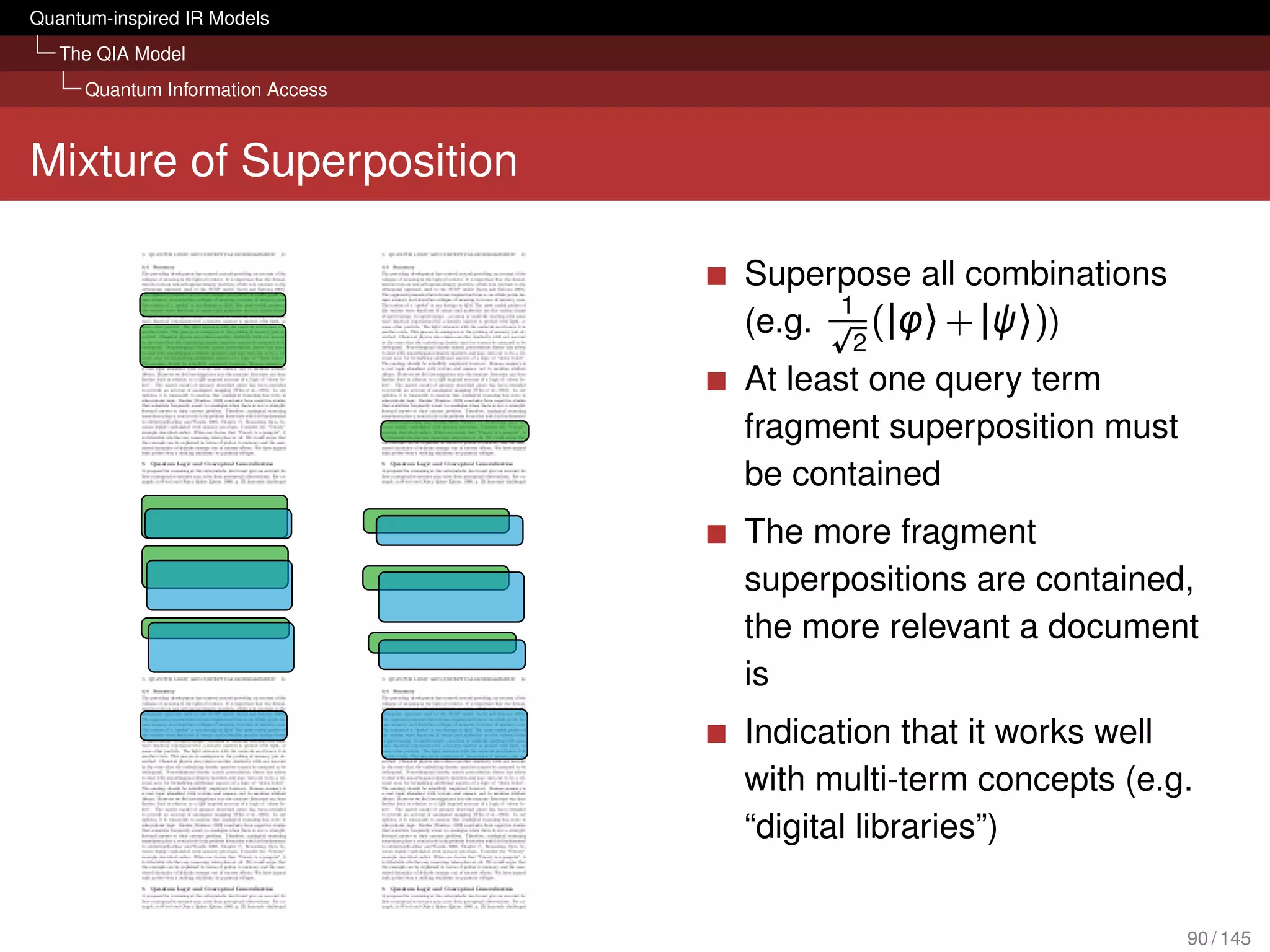
92. Quantum-inspired IR Models
The QIA Model
Quantum Information Access
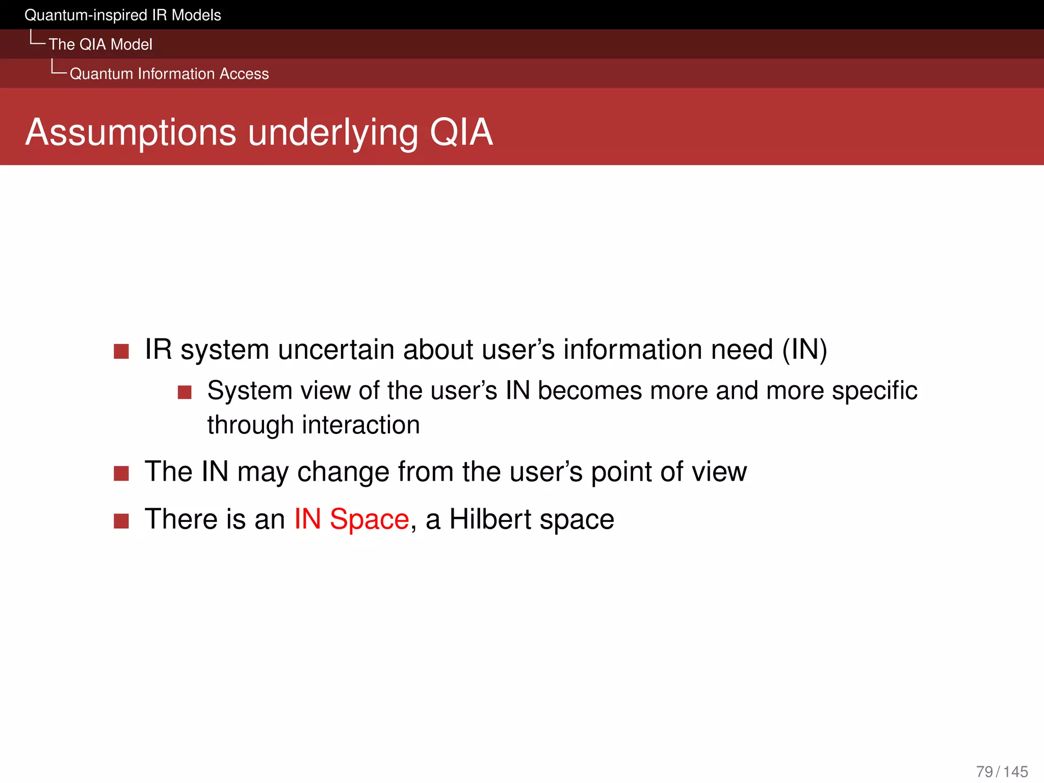
What can it bring to IR?
Evaluation with several TREC collections
[Piwowarski et al., 2010]
Tensor representation of query could compete with BM25
We don’t lose retrieval effectiveness in an ad hoc scenario
Framework is open for possible extension:
Different forms of interactions (query reformulations, relevance
judgements) sessions
Diversity and novelty
Structured queries (Boolean; based on mixture, superposition and
tensor)
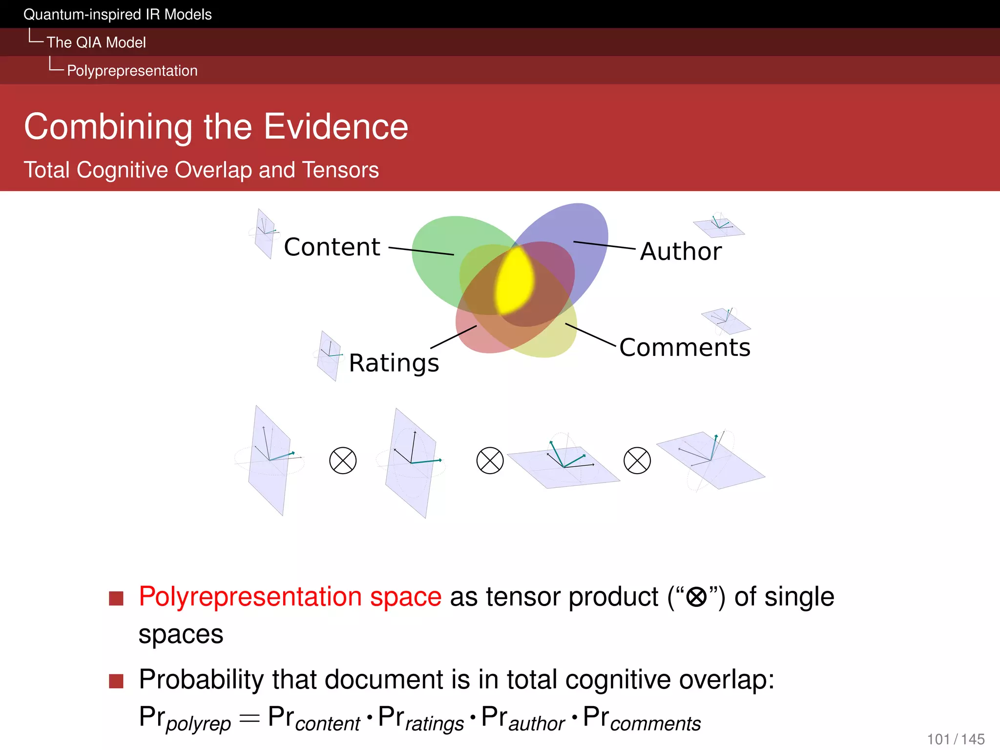
Polyrepresentation [Frommholz et al., 2010]
92 / 145

93. Quantum-inspired IR Models
The QIA Model
Polyprepresentation
Book Store Example
93 / 145

94. Quantum-inspired IR Models
The QIA Model
Polyprepresentation
Book Store Example
94 / 145

95. Quantum-inspired IR Models
The QIA Model
Polyprepresentation
The Principle of Polyrepresentation
Book Store Scenario
Content Author
Comments
Ratings
1 Get ranking for different representations
2 Find the cognitive overlap
Based on different document representations, but also different
representations of user’s information need
Hypothesis: cognitive overlap contains highly relevant documents
(experiments support this) 95 / 145

96. Quantum-inspired IR Models
The QIA Model
Polyprepresentation
How can we apply this in QIA?
Model single representations in a vector space (by example)
Authors
Ratings
Combine the representations
96 / 145

97. Quantum-inspired IR Models
The QIA Model
Polyprepresentation
Example: Author Space
Each author is a dimension
Non-orthogonal vectors:
dependencies
Angle between vectors
reflects the degree of
dependency (90◦ =
orthogonal = upright =
independent)
Example: Jones and Smith
(somehow) related, Smith and
Miller not
97 / 145

98. Quantum-inspired IR Models
The QIA Model
Polyprepresentation
Example: Author Space
Document by Smith and Miller
User seeks for documents by
Jones
Document retrieved due to
relationship between Jones
and Smith
98 / 145

99. Quantum-inspired IR Models
The QIA Model
Polyprepresentation
Rating Space
Example: rating scale
good/bad/average – each is a |average
dimension
|bad
“Average” rated book
represented by 2-dimensional |good
subspace
User wants books which are
rated good
⇒ not relevant (|good 〉
Rrating
orthogonal)
99 / 145

100. Quantum-inspired IR Models
The QIA Model
Polyprepresentation
Combining the Evidence
Total Cognitive Overlap and Tensors
Modelled different representations in vector space
Probabilities w.r.t. single representations
How do we express user’s IN w.r.t. all representations?
How do we get a cognitive overlap?
100 / 145

101. Quantum-inspired IR Models
The QIA Model
Polyprepresentation
Combining the Evidence
Total Cognitive Overlap and Tensors
Content Author
Comments
Ratings
Polyrepresentation space as tensor product (“⊗”) of single
spaces
Probability that document is in total cognitive overlap:
Prpolyrep = Prcontent · Prratings · Prauthor · Prcomments
101 / 145

102. Quantum-inspired IR Models
The QIA Model
Polyprepresentation
Wishlist
Content Author
Comments
Ratings
Documents not relevant in one representation should not get a
value of 0
Ignore selected representations
Relative importance of representations to user (mixing and
weighting)
102 / 145

103. Quantum-inspired IR Models
The QIA Model
Polyprepresentation
“Don’t care” dimension
Introduction of a “don’t care” dimension
Part of each document subspace
each document “satisfies” the don’t care “need”
Example: Document by Smith, user doesn’t care about authors
with probability α
|jones
|smith Rauthor
α
|∗
α = 1 means representation is ignored at all
103 / 145

104. Quantum-inspired IR Models
The QIA Model
Polyprepresentation
Example
What the system assumes about the user’s IN:
Seeks books either by Jones or by Smith
Looks either for good books or doesn’t care about ratings
Assume a document d by Smith which is rated “bad”
Polyrepresentation space: 9-dimensional (3 × 3)
104 / 145

105. Quantum-inspired IR Models
The QIA Model
Polyprepresentation
IN Vectors in Polyrepresentation Space
How do they look like and what do they mean?
Reflects all 4 possible
combinations of INs w.r.t. single
representations:
Smith/good: |smith 〉 ⊗ |good 〉
Smith/dont’ care: |smith 〉 ⊗ |∗〉
Jones/good: |jones 〉 ⊗ |good 〉
Jones/dont’ care: |jones 〉 ⊗ |∗〉
Polyrepresentation space
105 / 145

106. Quantum-inspired IR Models
The QIA Model
Polyprepresentation
Documents in Polyrepresentation Space
Represented as tensor product of single document subspaces
Here: 4-dimensional subspace (2 × 2)
106 / 145

107. Quantum-inspired IR Models
The QIA Model
Polyprepresentation
Determining the Retrieval Weight
Why the system retrieves the
bad book by Smith
107 / 145

108. Quantum-inspired IR Models
The QIA Model
Polyprepresentation
Something left on the Wishlist
Relationships between Representations
System observes (interaction/feedback) user preferences:
If book is by Smith, it has to be rated good
If book is by Jones, don’t care about the ratings
System evolves to new state in polyrepresentation space (2
combinations not allowed any more)
X
X
108 / 145

109. Quantum-inspired IR Models
The QIA Model
Polyprepresentation
What does that mean?
Only two assumed IN
cases left:
1 Smith/good
2 Jones/don’t care
Cannot be expressed as
combination of single
representations
Bad book by Smith only
retrieved due to
relationship to Jones!
109 / 145

110. Quantum-inspired IR Models
The QIA Model
Polyprepresentation
QIA Summary
We showed how we can express polyrepresentation in a mathematical
framework inspired by quantum mechanics:
Presented IN space
Modelled different example representations
Combined representations in polyrepresentation space
110 / 145

111. Quantum-inspired IR Models
The QIA Model
Polyprepresentation
QIA Conclusion
QIA framework
User’s IN as ensemble of vectors
Documents as subspaces
User interaction and feedback
Term space, query construction
Can compete in an ad hoc scenario
Polyrepresentation
Different non-topical representations as subspaces
Polyrepresentation space as tensor space to calculate cognitive
overlap
“Don’t care” dimension for weighting of representations
Non-separate states reflect interdependencies
111 / 145

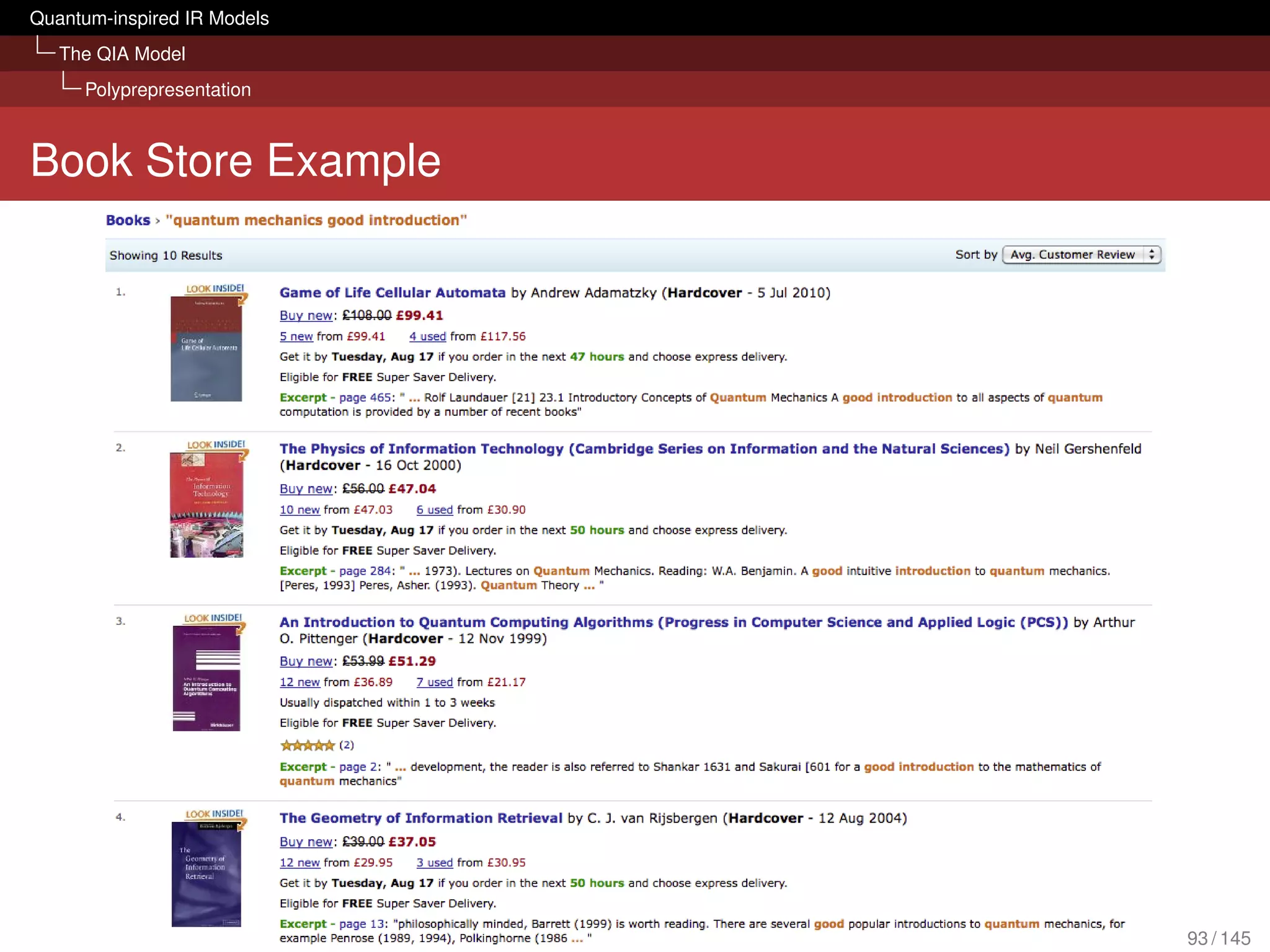
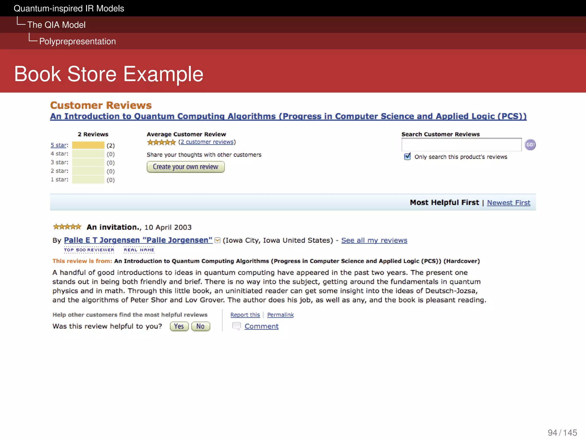
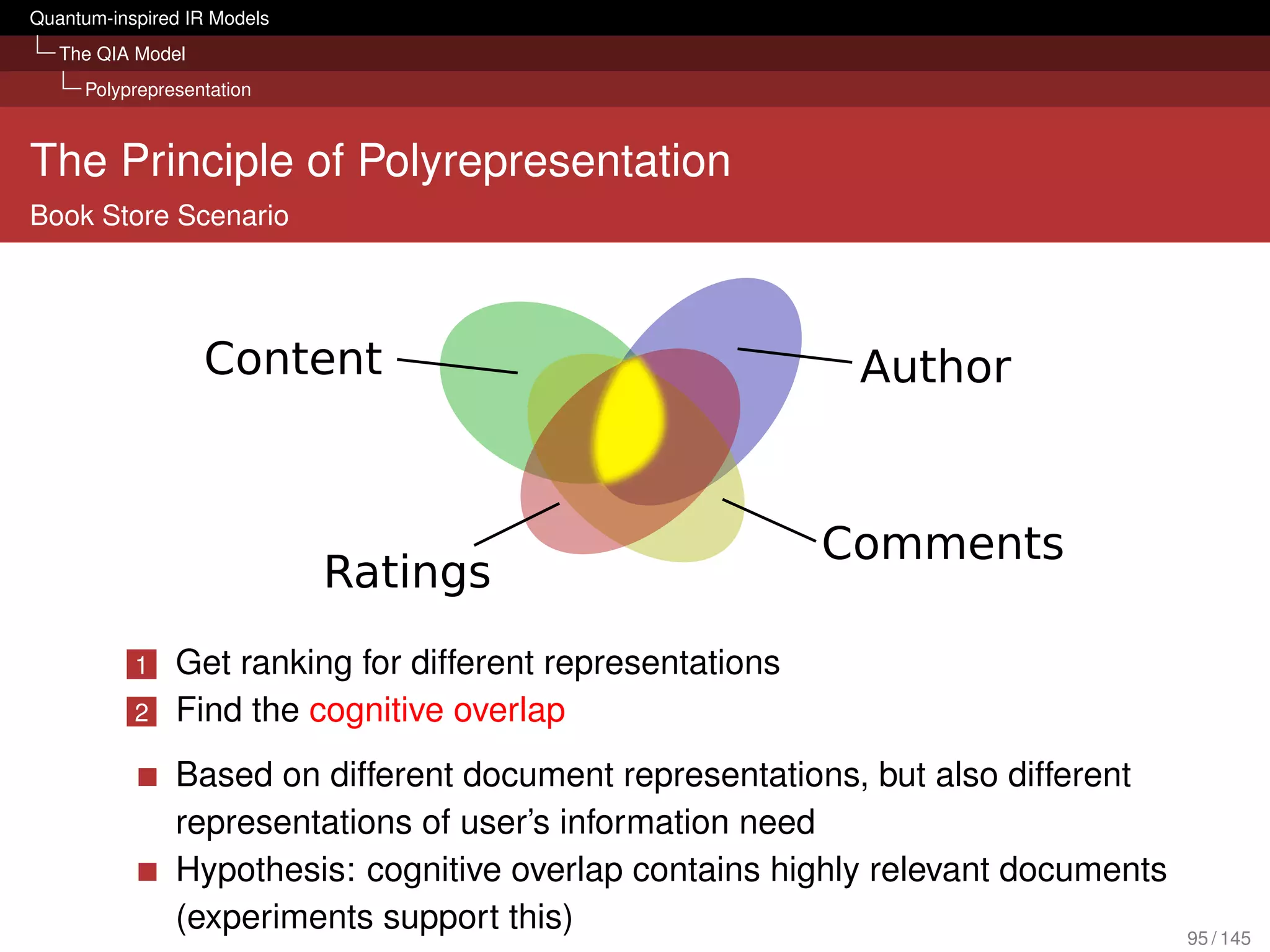
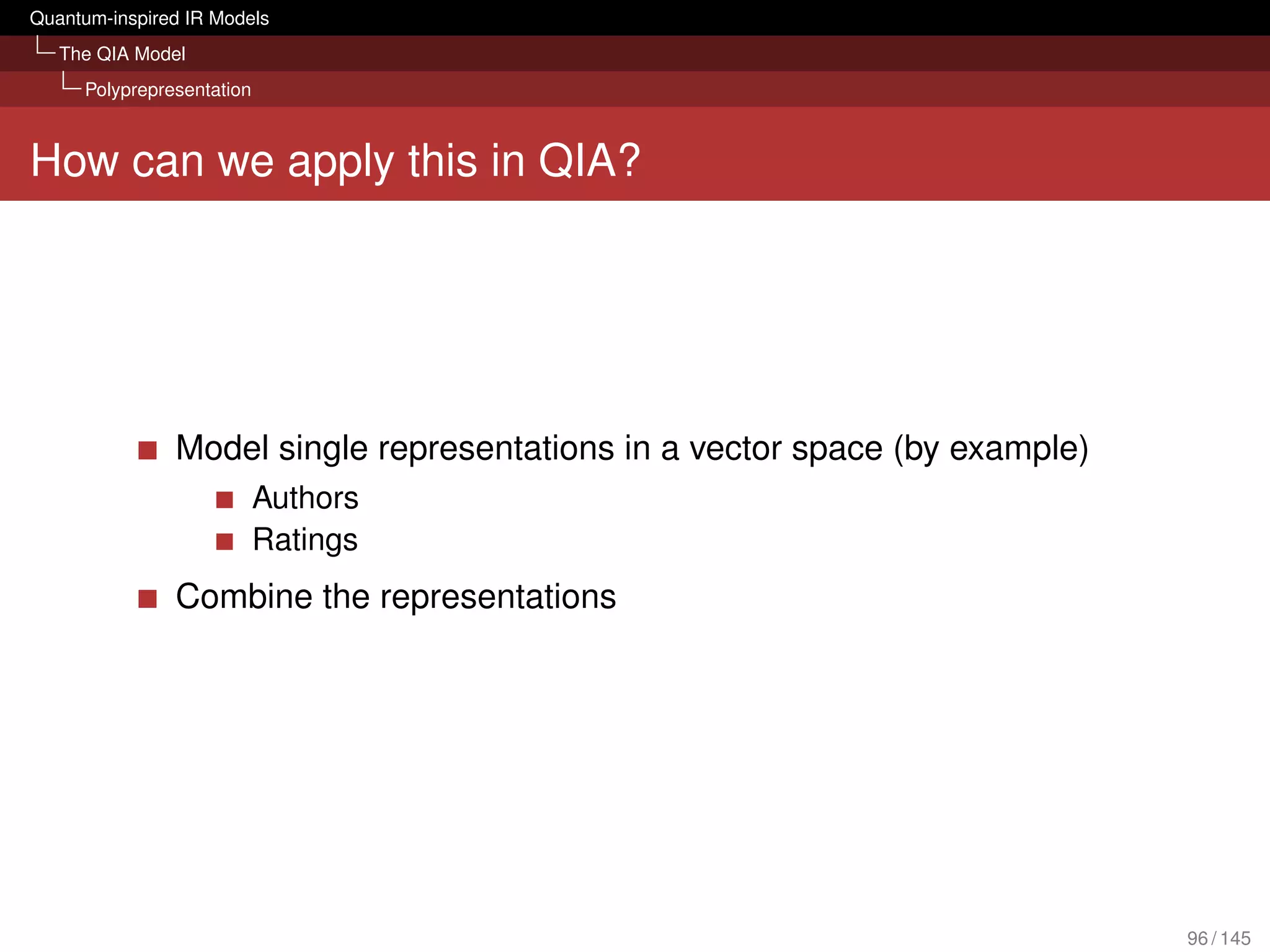
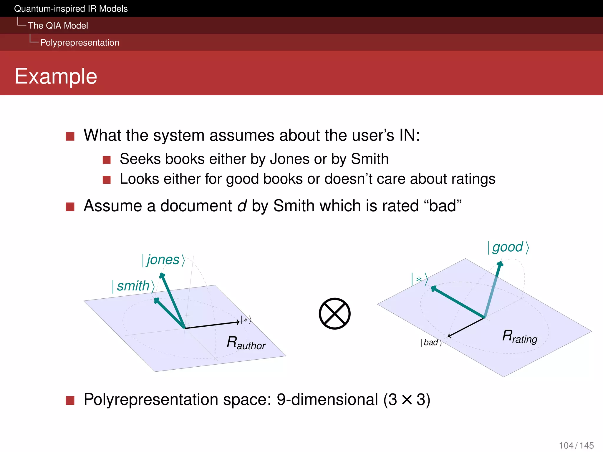
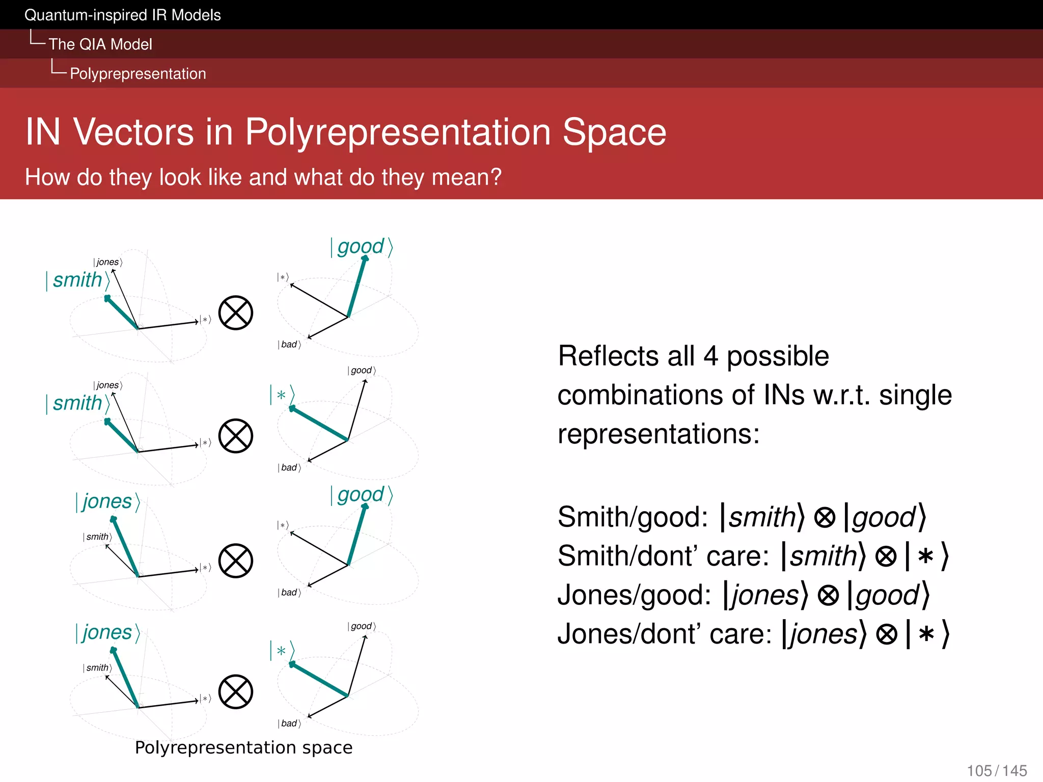
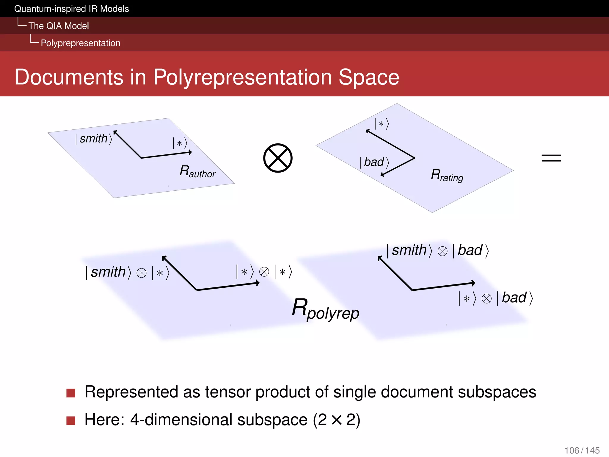
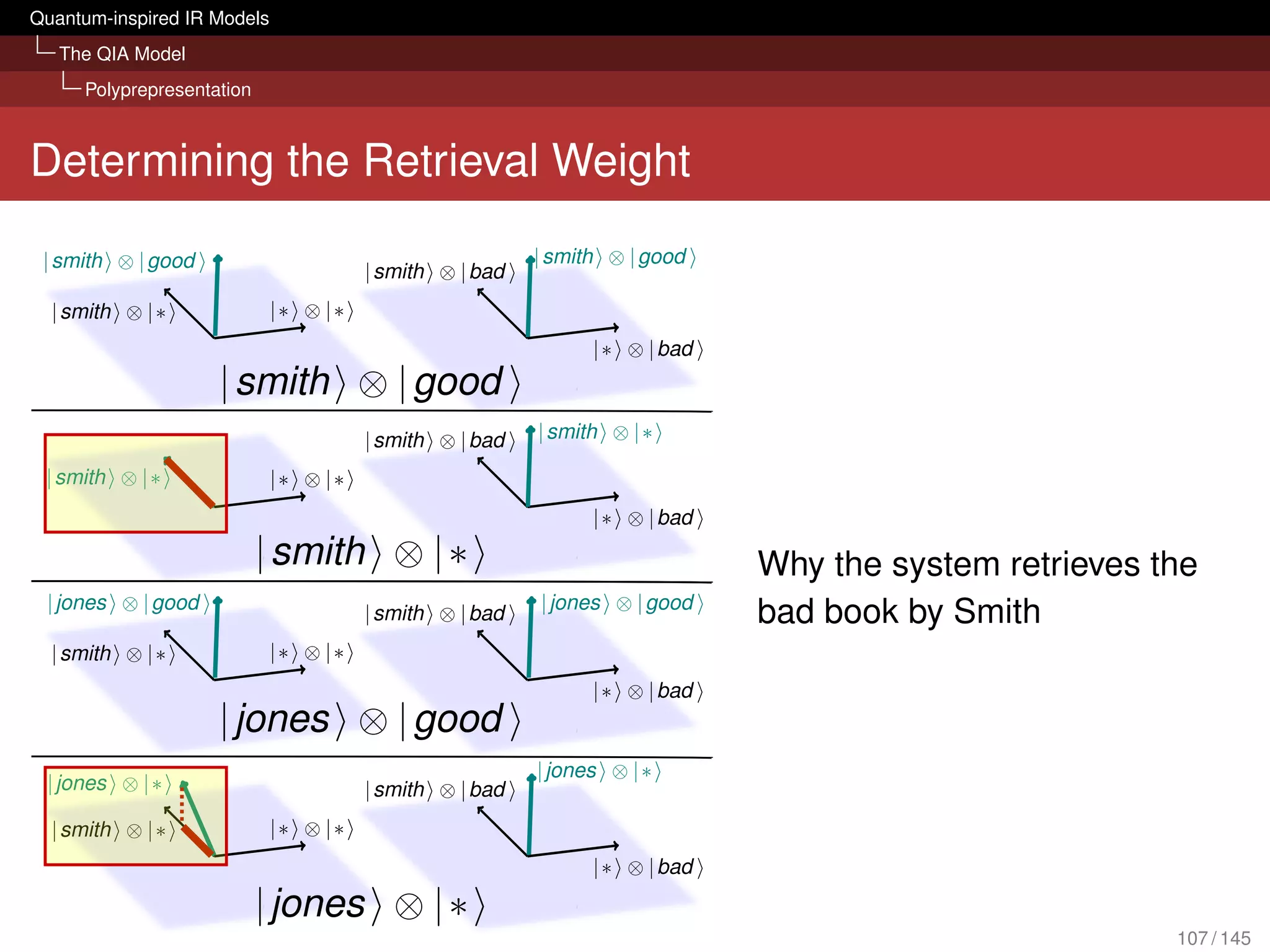
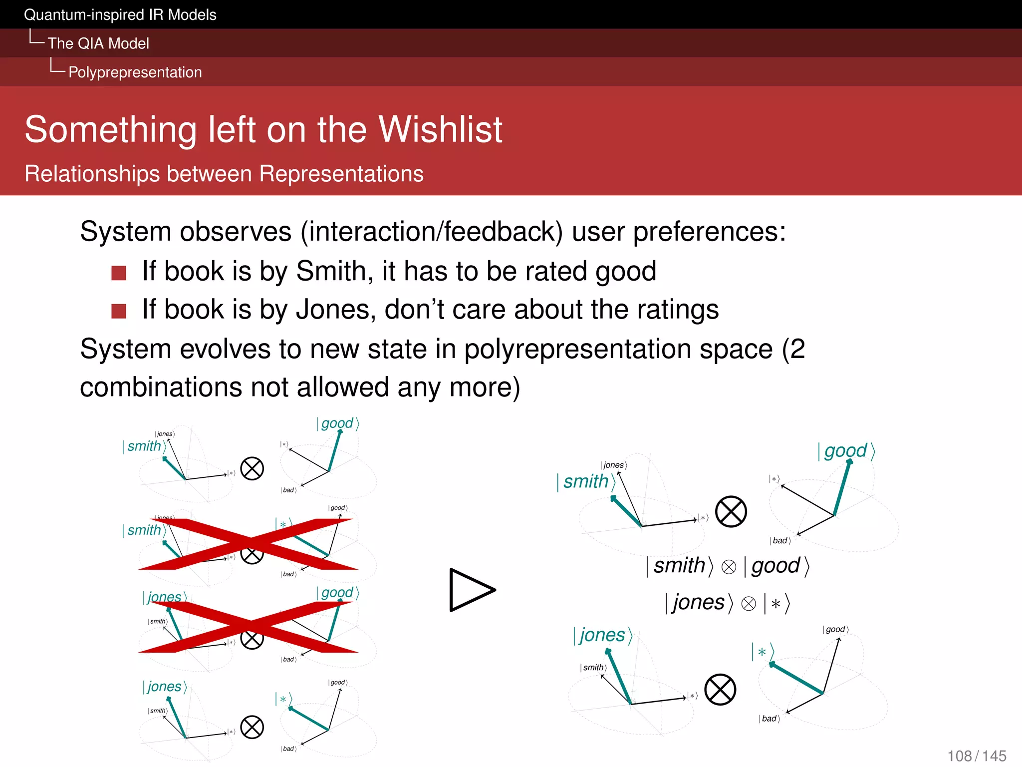
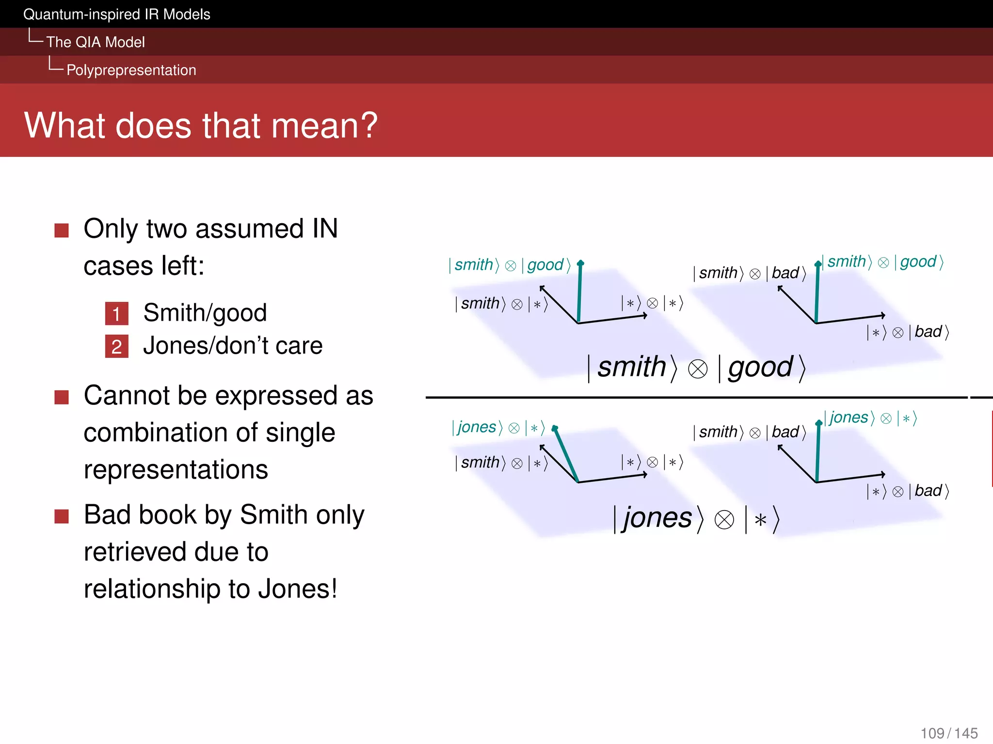
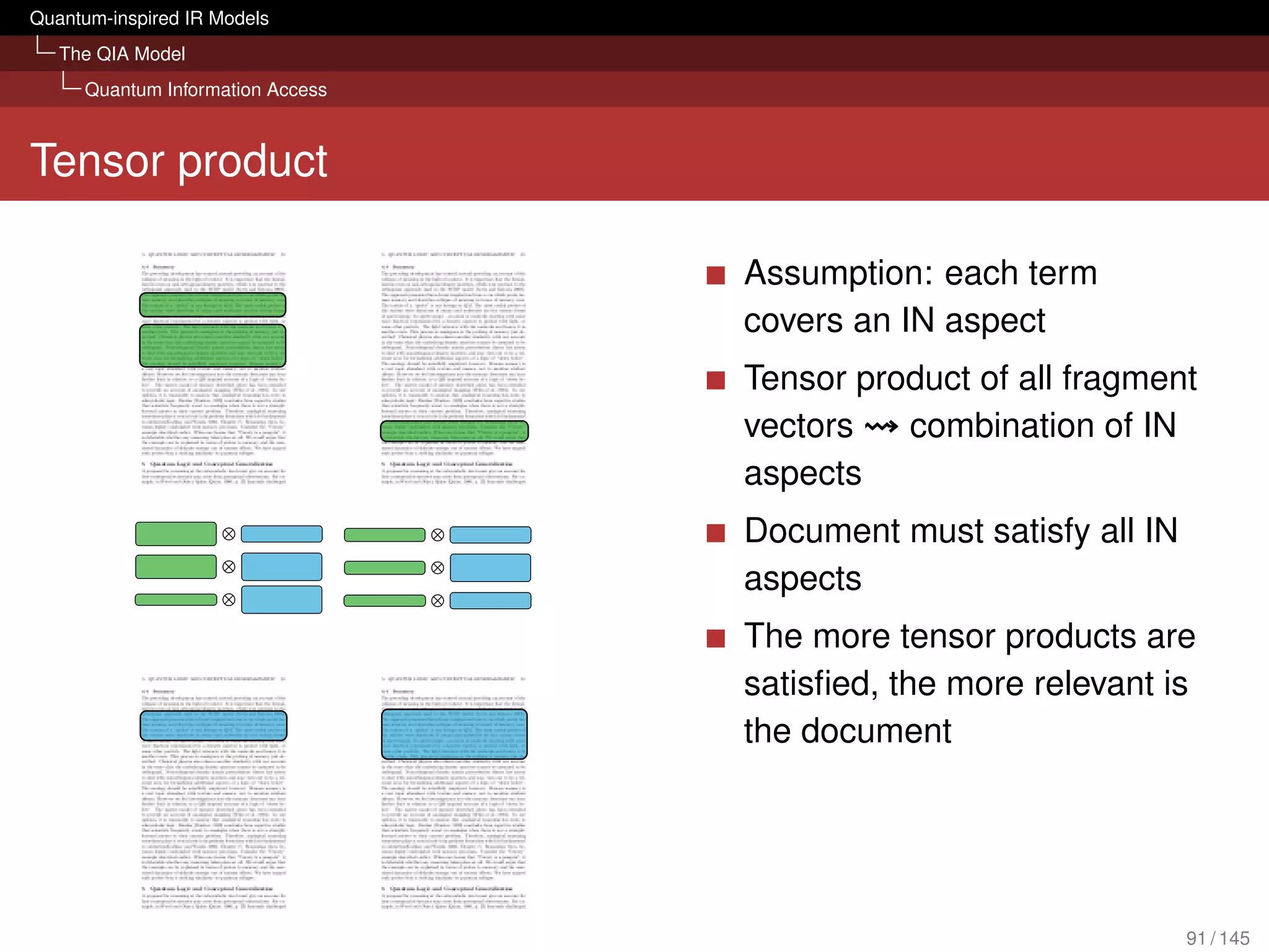
112. Quantum-inspired IR Models
The QIA Model
Polyprepresentation
QIA Extensions
Queries in sessions [Frommholz et al., 2011]
Use geometry and projections to determine type of and handle
follow-up query (generalisation, information need drift,
specialisation)
Summarisation [Piwowarski et al., 2012]
QIA interpretation of LSA-based methods
Query algebra for the QIA framework [Caputo et al., 2011]
112 / 145

113. The Quantum Probability Ranking Principle (qPRP) [Zuccon, 2012]

114. Quantum-inspired IR Models
Quantum Probability Ranking Principle
Quantum Interference (again)
Recall the double slit experiment
Probability amplitudes instead of
probabilities to model interference
Derived the interference term
I = ϕ1 ϕ2 + ϕ2 ϕ1
= 2· Pr1 (x ) Pr2 (x ) · cos(θ1 − θ2 )
to compute
Pr12 (x ) = Pr1 (x ) + Pr2 (x ) + I
114 / 145

115. Quantum-inspired IR Models
Quantum Probability Ranking Principle
Probability Ranking Principle
Probability Ranking Principle (PRP): Rank according to
decreasing Pr(R |d , q )
Which document to present next?
argmax (Pr (R |d , q ))
d ∈B
B : candidate documents not presented yet
Assumes relevance judgements are independent, no
dependencies between documents
Potentially does not suit tasks considering novelty and diversity
well!
115 / 145

116. Quantum-inspired IR Models
Quantum Probability Ranking Principle
Quantum Probability Ranking Principle
Double Slit Analogy
4.4 Ranking Documents within the Analogy
IR analogy to double slit experiment
User is “particle” dA dA
Each slit corresponds to a
pd A d B
document
Event that particle passes through d B? dB
slit: user analyses document
Screen measures user satisfaction B
(proportional to Pr(R |d , q )) d B1 ... d Bi ... d Bn 1
Which document to present next
(after user saw dA )? Figure 4.6: The IR analogous of the situation pictured in Figure 4.5.
(taken from [Zuccon, 2012])
pdA dB : there is no reason for which to expect that pdA dBi = pdA dBj , 8dBi , dBj 2 B.
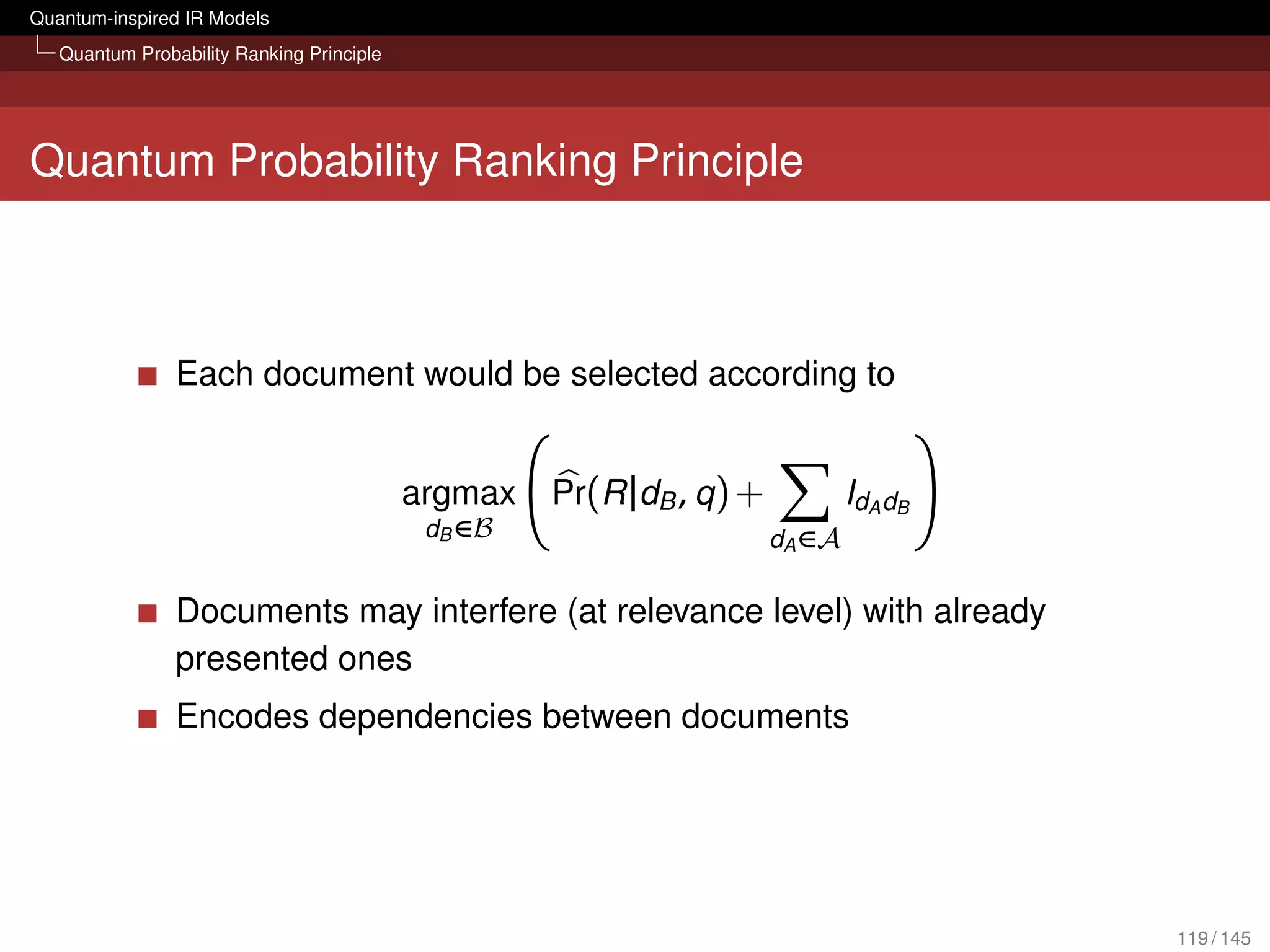
argmax Pr (R |dB , q ) + IdA dB
A question now arises: which document (slit) dB 2 B should be selected such
that, once coupled with document (slit) dA , the probability pdA dB is maximised?
dB ∈B Answering this question corresponds to define a criteria for selecting documents
such that, once coupled with the already ranked document, the likelihood of de-
livering maximum satisfaction to the user is maximised. In terms of the physical
experiment, this would correspond to selecting slits among the set116 / 145
of available

117. Quantum-inspired IR Models
Quantum Probability Ranking Principle
Quantum Probability Ranking Principle
Assumptions
1 Ranking is performed sequentially
2 Empirical data is best described by quantum probabilities
3 Relevance of documents not assessed in isolation;
documents that have been ranked before influence future
relevance assessments
117 / 145

118. Quantum-inspired IR Models
Quantum Probability Ranking Principle
Quantum Probability Ranking Principle (qPRP)
Let A (where A = ∅ is also considered) be the set containing the
documents that have been already retrieved until rank i − 1 and let B
be the set of candidate documents for being retrieved at rank i. In
order to maximise its effectiveness, an Information Retrieval system
has to rank document dB ∈ B at rank i if and only if
Pr(R |dB , q ) + IdA dB ≥ Pr(R |dC , q ) + IdA dC ,
for any dC ∈ B . IdA dB is the sum of the quantum interference terms
produced considering all the pairs composed by dB and each already
retrieved document dA ∈ A (similarly for IdA dC ).
118 / 145

119. Quantum-inspired IR Models
Quantum Probability Ranking Principle
Quantum Probability Ranking Principle
Each document would be selected according to
argmax Pr(R |dB , q ) + IdA dB
dB ∈B dA ∈A
Documents may interfere (at relevance level) with already
presented ones
Encodes dependencies between documents
119 / 145

120. Quantum-inspired IR Models
Quantum Probability Ranking Principle
qPRP: Interference Term
Estimation
Recall
IdA dB = ϕdA ϕdB + ϕdB ϕdA
= 2· Pr(R |dA , q ) Pr(R |dB , q ) · cos(θAB )
(with cos(θAB ) = cos(θdA − θdB ))
Interference governed by the phase difference θAB between
ϕdA ∈ C and ϕdB ∈ C
Destructive: cos(θAB ) < 0
Constructive: cos(θAB ) > 0
Estimate IdA dB with similarity function fsim
cos(θAB ) ≈ βfsim (dA , dB )
β ∈ R: normalisation, sign of interference
120 / 145

121. Quantum-inspired IR Models
Quantum Probability Ranking Principle
qPRP: Evaluation
Different similarity functions applied in diversity task (TREC 6,7,8
and ClueWeb B)
qPRP outperformed PRP and (sometimes) a Portfolio Theory
setting (but no parameter tuning required)
Kullback-Leibler divergence performed best
Pearson’s correlation coefficient seems most robust
121 / 145

122. Quantum-inspired IR Models
Quantum Probability Ranking Principle
qPRP: Evaluation
Further Experiments
Comparison with PRP, Maximal Marginal relevance (MMR),
Portfolio Theory (PT) and interactive PRP (iPRP)
Ad hoc task
PRP best performing ranking approach when independence
assumption hold
Diversity task
PRP often outperformed by PT, iPRP and qPRP
122 / 145

123. Quantum-inspired IR Models
Quantum Probability Ranking Principle
qPRP: Discussion
Kolmogorovian probabilities (in PRP) adequate when using
independence assumption (ad hoc task)
Quantum probabilities seem good choice if documents are not
independent and interfere (diversity task)
qPRP reduces to PRP if phases are perpendicular
(cos(θAB ) = 0)
Integration into QIA framework possible
123 / 145

124. Further Models and Conclusion
Further Work and Software
Discussion and Conclusion

125. Further Models and Conclusion
Further Work and Software
Further Selected Works
Quantum probability in context [Melucci, 2008]
Effective query expansion with quantum interference
[Melucci, 2010b]
Semantics and meaning [Widdows, 2004]
Entanglement and word meaning
[Bruza et al., 2009b, Bruza et al., 2009a]
Lattice structures and documents [Huertas-Rosero et al., 2009]
Quantum theory and search [Arafat, 2007]
Query expansion and query drift [Zhang et al., 2011]
Document re-ranking [Zhao et al., 2011]
Complex numbers in IR [Zuccon et al., 2011]
DB+IR: Commutative Quantum Query Language [Schmitt, 2008]
Further overview [Song et al., 2010]
125 / 145

126. Further Models and Conclusion
Further Work and Software
Software
Kernel Quantum Probability API by Benjamin Piwowarski
http://kqp.bpiwowar.net/
126 / 145

127. Further Models and Conclusion
Further Work and Software
Other Resources
http://www.quantuminteraction.org/home
A collection of useful links and resources in the context of the
Quantum Interaction series
http://www.mendeley.com/groups/496611/
quantum-and-geometry-ir/
Aiming at providing an updated list of quantum and geometry IR
research papers
You may also follow me on Twitter: @iFromm
127 / 145

128. Further Models and Conclusion
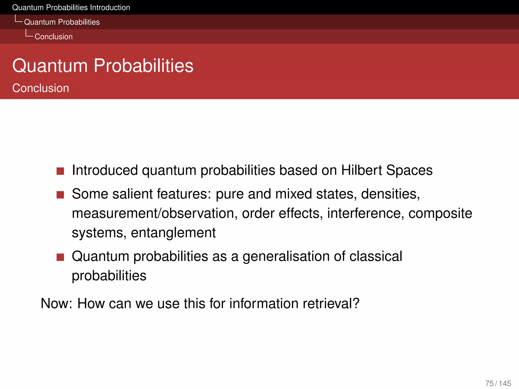
Discussion and Conclusion
Discussion
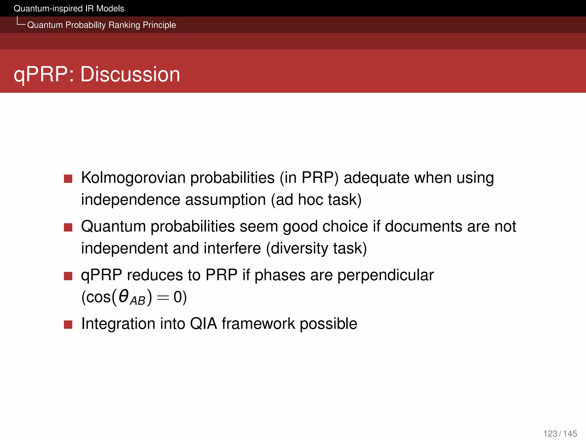
Quantum Theory and IR
The quantum formalism is a powerful ’language’ for IR – isn’t it?
We’ve seen some examples of quantum-inspired models (QIA,
qPRP)
Quantum probabilities may give us a hint of what is wrong with
existing approaches (but not always!) [Piwowarski et al., 2012]
But there is criticism: “Ornamental but not useful” (Kantor, who
hopes to be proven wrong) [Kantor, 2007]
128 / 145

129. Further Models and Conclusion
Discussion and Conclusion
Conclusion
Quantum probabilities
2 quantum-inspired approaches: QIA and qPRP
Further approaches
129 / 145

130. Questions?

131. Bibliography
Bibliography I
Aerts, D. and Gabora, L. (2005).
A theory of concepts and their combinations II: A Hilbert space
representation.
Kybernetes, 34(1/2):192–221.
Arafat, S. (2007).
Foundations Research in Information Retrieval Inspired by
Quantum Theory.
Phd thesis, University of Glasgow.
131 / 145

132. Bibliography
Bibliography II
Bruza, P., Kitto, K., Nelson, D., and McEvoy, C. (2009a).
Extracting Spooky-Activation-at-a-Distance from Considerations
of Entanglement.
In Proc. of the Third Quantum Interaction Symposium (QI 2009),
volume 5494 of Lecture Notes in Computer Science, pages
71–83, Berlin, Heidelberg. Springer Berlin Heidelberg.
Bruza, P., Kitto, K., Nelson, D., and McEvoy, C. (2009b).
Is there something quantum-like about the human mental lexicon?
Journal of mathematical psychology, 53(5):363–377.
132 / 145

133. Bibliography
Bibliography III
Busemeyer, J. R. (2012).
Introduction to Quantum Probability for Social and Behavioral
Scientists.
In Rudolph, L. and Valsiner, J., editors, Qualitative Mathematics
for Social Sciences - Mathematical Models for Research on
Cultural Dynamics. Routledge.
Caputo, A., Piwowarski, B., and Lalmas, M. (2011).
A Query Algebra for Quantum Information Retrieval.
In Proceedings of the 2nd Italian Information Retrieval Workshop
2011.
133 / 145

134. Bibliography
Bibliography IV
Di Buccio, E., Melucci, M., and Song, D. (2011).
Towards Predicting Relevance Using a Quantum-Like Framework.
In Clough, P., Foley, C., Gurrin, C., Jones, G. J. F., Kraaij, W., Lee,
H., and Mudoch, V., editors, Proceedings ECIR 2011, volume
6611 of Lecture Notes in Computer Science, pages 755–758.
Springer.
Feynman, R. P. (1951).
The Concept of Probability in Quantum Mechanics.
In Proc. Second Berkeley Symp. on Math. Statist. and Prob. (Univ.
of Calif. Press, 1951), pages 533–541.
134 / 145

135. Bibliography
Bibliography V
Frommholz, I., Larsen, B., Piwowarski, B., Lalmas, M., Ingwersen,
P., and van Rijsbergen, K. (2010).
Supporting Polyrepresentation in a Quantum-inspired Geometrical
Retrieval Framework.
In Proceedings of the 2010 Information Interaction in Context
Symposium, pages 115–124, New Brunswick. ACM.
Frommholz, I., Piwowarski, B., Lalmas, M., and van Rijsbergen, K.
(2011).
Processing Queries in Session in a Quantum-Inspired IR
Framework.
In Clough, P., Foley, C., Gurrin, C., Jones, G. J. F., Kraaij, W., Lee,
H., and Mudoch, V., editors, Proceedings ECIR 2011, volume
135 / 145

136. Bibliography
Bibliography VI
6611 of Lecture Notes in Computer Science, pages 751–754.
Springer.
Griffiths, R. B. (2002).
Consistent quantum theory.
Cambridge University Press, Cambridge; New York.
Halmos, P. R. (1958).
Finite-Dimensional Vector Spaces.
Springer-Verlag New York Heidelberg Berlin.
Huertas-Rosero, A., Azzopardi, L., and van Rijsbergen, C. J.
(2009).
Eraser Lattices and Semantic Contents.
In Proceedings Quantum Interaction 2009, pages 266–275.
136 / 145

137. Bibliography
Bibliography VII
Hughes, R. (1992).
The Structure and Interpretation of Quantum Mechanics.
Harvard University Press.
Kantor, P. B. (2007).
Keith van Rijsbergen, The Geometry of Information Retrieval.
Information Retrieval, 10(4-5):485–489.
Melucci, M. (2008).
A basis for information retrieval in context.
ACM Transactions on Information Systems (TOIS), 26(3).
137 / 145

138. Bibliography
Bibliography VIII
Melucci, M. (2010a).
An Investigation of Quantum Interference in Information Retrieval.
In Cunningham, H., Hanbury, A., and Rüger, S., editors,
Proceedings of the First Information Retrieval Facility Conference
(IRFC 2010), pages 136–151. Springer.
Melucci, M. (2010b).
An Investigation of Quantum Interference in Information Retrieval.
In Cunningham, H., Hanbury, A., and Rüger, S., editors,
Proceedings of the First Information Retrieval Facility Conference
(IRFC 2010), pages 136–151. Springer.
138 / 145

139. Bibliography
Bibliography IX
Melucci, M. and Rijsbergen, K. V. (2011).
Quantum Mechanics and Information Retrieval.
In Melucci, M. and Baeza-Yates, R., editors, Advanced Topics in
Information Retrieval, volume 33 of The Information Retrieval
Series, chapter 6, pages 125–154. Springer Berlin Heidelberg,
Berlin, Heidelberg.
Nielsen, M. A. and Chuang, I. L. (2000).
Quantum Computation and Quantum Interaction.
Cambridge University Press, Cambridge, UK.
139 / 145

140. Bibliography
Bibliography X
Piwowarski, B., Amini, M.-R., and Lalmas, M. (2012).
On using a Quantum Physics formalism for Multi-document
Summarisation.
Journal of the American Society for Information Science and
Technology (JASIST).
Piwowarski, B., Frommholz, I., Lalmas, M., and Van Rijsbergen, K.
(2010).
What can Quantum Theory Bring to Information Retrieval?
In Proc. 19th International Conference on Information and
Knowledge Management, pages 59–68. Springer.
140 / 145

141. Bibliography
Bibliography XI
Piwowarski, B. and Lalmas, M. (2009).
A Quantum-based Model for Interactive Information Retrieval.
In Proceedings of the 2nd International Conference on the Theory
of Information Retrieval (ICTIR 2009), Cambridge, UK.
Schmitt, I. (2008).
QQL : A DB&IR Query Language.
The VLDB Journal, 17(1):39–56.
Song, D., Lalmas, M., van Rijsbergen, K., Frommholz, I.,
Piwowarski, B., Wang, J., Zhang, P., Zuccon, G., Bruza, P., Arafat,
S., Azzopardi, L., Huertas-Rosero, A., Hou, Y., Melucci, M., and
Rüger, S. (2010).
How Quantum Theory is Developing the Field of Information
Retrieval.
141 / 145

142. Bibliography
Bibliography XII
In Proceedings Quantum Interaction 2010.
Song, D., Melucci, M., Frommholz, I., Zhang, P., Wang, L., and
Arafat, S., editors (2011).
Quantum Interaction: 5th International Symposium, QI 2011,
Aberdeen, UK, Revised Selected Papers.
Springer Berlin Heidelberg, lecture no edition.
van Rijsbergen, C. J. (2004).
The Geometry of Information Retrieval.
Cambridge University Press, New York, NY, USA.
Widdows, D. (2004).
Geometry and Meaning.
Center for the Study of Language and Information, Stanford
University.
142 / 145

143. Bibliography
Bibliography XIII
Zhang, P., Song, D., Zhao, X., and Hou, Y. (2011).
Investigating Query-Drift Problem from a Novel Perspective of
Photon Polarization.
In Amati, G. and Crestani, F., editors, Advances in Information
Retrieval Theory - Proc. of ICTIR 2011, pages 332–336. Springer.
Zhao, X., Zhang, P., Song, D., and Hou, Y. (2011).
A Novel Re-ranking Approach Inspired by Quantum
Measurement.
In Clough, P., Foley, C., Gurrin, C., Jones, G. J. F., Kraaij, W., Lee,
H., and Mudoch, V., editors, Proceedings ECIR 2011, volume
6611 of Lecture Notes in Computer Science, pages 721–724.
Springer.
143 / 145

144. Bibliography
Bibliography XIV
Zuccon, G. (2012).
Document Ranking with Quantum Probabilities.
Phd thesis, University of Glasgow.
Zuccon, G., Azzopardi, L., and van Rijsbergen, K. (2009).
The Quantum Probability Ranking Principle for Information
Retrieval.
In Advances in Information Retrieval Theory - Proc. of ICTIR
2009, volume 5766 of Lecture Notes in Computer Science, pages
232–240, Berlin, Heidelberg. Springer Berlin Heidelberg.
144 / 145

145. Bibliography
Bibliography XV
Zuccon, G., Piwowarski, B., and Azzopardi, L. (2011).
On the use of Complex Numbers in Quantum Models for
Information Retrieval.
In Amati, G. and Crestani, F., editors, Advances in Information
Retrieval Theory - Proc. of ICTIR 2011, pages 346–350. Springer.
145 / 145