Download as PDF, PPTX
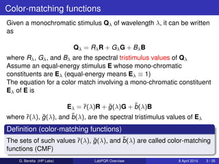
![CIE 1931 standard colorimetric observer
We want to build an instrument delivering results valid for the group of
normal trichromats (95% of population); since
R=k Pλ¯(λ)dλ
r
G=k ¯
Pλ g (λ)dλ
B=k ¯
Pλ b(λ)dλ
an ideal observer can be defined by specifying values for the
color-matching functions
Definition (CIE 1931 standard colorimetric observer)
The Commission Internationale de l’Éclairage (CIE) has recommended
¯ ¯ ¯
such tables containing x (λ), y (λ), z (λ) for λ ∈ [360nm, 830nm] in 1nm
steps
G. Beretta (HP Labs) LabPQR Overview 8 April 2010 5 / 35](https://image.slidesharecdn.com/labpqr-12720685223879-phpapp02/85/The-LabPQR-Color-Space-5-320.jpg)
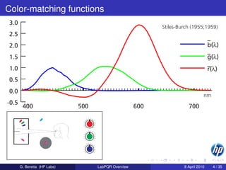
![Discretization
In practice, the CMF are given as a table with 1nm steps, and
instruments measure at steps of 1, 4, 10, 20nm etc., so in reality this is
a summation [for red R]:
R=k ¯(λ)E(λ)S(λ)dλ ≈ k
r ¯(λi )E(λi )S(λi )∆λ
r
The integration resp. summation is over the visible range [380, 780]nm,
but in practice it is often over [380, 730]nm for n = 36 samples
Instead of doing color science with measure theory, we can do it
with simple linear algebra
In 1991 H. Joel Trussell has made available a comprehensive
MatLab library and several key papers for color scientists
Since then, spectral color science is mostly done with linear
algebra
G. Beretta (HP Labs) LabPQR Overview 8 April 2010 8 / 35](https://image.slidesharecdn.com/labpqr-12720685223879-phpapp02/85/The-LabPQR-Color-Space-8-320.jpg)
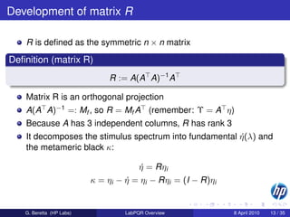
![Corollaries
Metameric black has tristimulus value zero
A κ = [0, 0, 0]
η = Rηi means that any group of metamers has a common
´
fundamental η , but different residues κ
´
Inversely, a stimulus spectrum can be expressed as
ηi = η + κ = Rηi + (I − R)ηi
´
i.e., the stimulus spectrum can be reconstructed if the
fundamental metamer and metameric black are known
Why is this useful?
G. Beretta (HP Labs) LabPQR Overview 8 April 2010 14 / 35](https://image.slidesharecdn.com/labpqr-12720685223879-phpapp02/85/The-LabPQR-Color-Space-14-320.jpg)

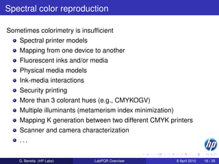
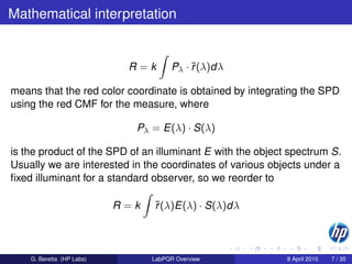
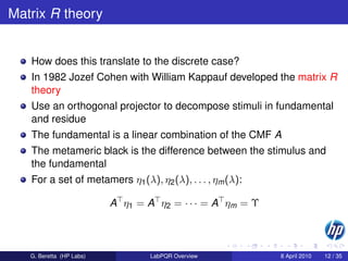
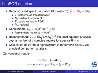
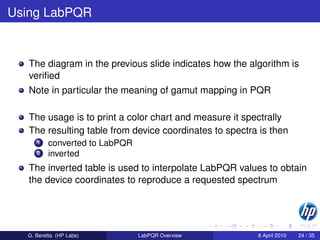
![The hard problem
We would like to use an ICC type workflow also for spectral
imaging
Colorimetric workflow:
profile connection
image 3-hue printer
space
The killer is the LUT used in the PCS:
bands in bands out levels per band size [bytes]
3 6 17 30K
6 6 17 145M
9 6 17 700G
31 6 17 8 · 1027 G
G. Beretta (HP Labs) LabPQR Overview 8 April 2010 18 / 35](https://image.slidesharecdn.com/labpqr-12720685223879-phpapp02/85/The-LabPQR-Color-Space-18-320.jpg)
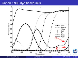
![Caveats
Green and black dyes tend to have an increasing reflectance in
the far red
Paper brighteners act in the blue range
RIT work: [400, 700]nm for n = 31 samples
Most real world data: [380, 730]nm for n = 36 samples
Visible range: [380, 780]nm
The range has a strong effect on the principal components
G. Beretta (HP Labs) LabPQR Overview 8 April 2010 26 / 35](https://image.slidesharecdn.com/labpqr-12720685223879-phpapp02/85/The-LabPQR-Color-Space-26-320.jpg)
![Accuracy of Matrix R vs. unconstrained
What price in loss of accuracy do we pay for compatibility
conventional metamerism theory?
Constrained model depends only on CMF
Unconstrained model additionally depends on device
Based on simulations (no LUT),
the constrained model is more accurate in general
for a single fixed printer, the unconstrained method allows the use
of less principal components: LabPQ
Short spectral range [400, 700]nm caused problems with green ink
G. Beretta (HP Labs) LabPQR Overview 8 April 2010 29 / 35](https://image.slidesharecdn.com/labpqr-12720685223879-phpapp02/85/The-LabPQR-Color-Space-29-320.jpg)


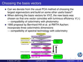
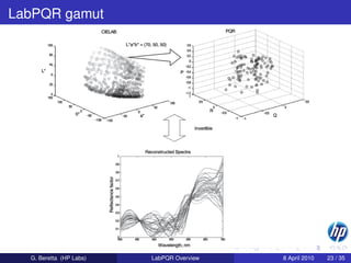
The document summarizes the LabPQR color space model proposed by researchers at Rochester Institute of Technology. The model uses a transformation from tristimulus values and a set of basis vectors derived from principal component analysis to represent color spectra in a lower dimensional space. This representation allows spectral data to be compressed while maintaining accuracy for applications like multi-spectral color reproduction. The model builds on prior work using matrix algebra to decompose color stimuli into fundamental and residue components.