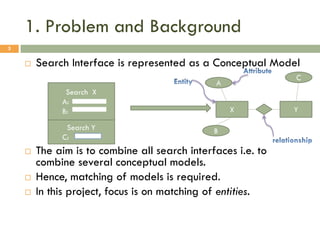
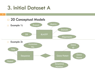
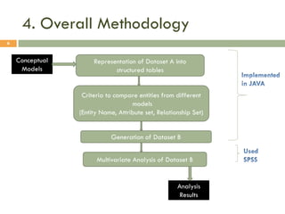
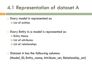
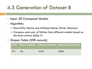
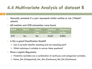
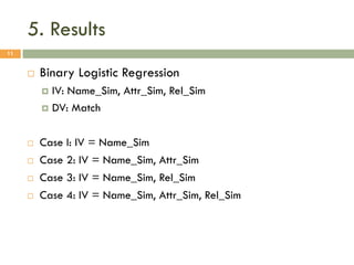
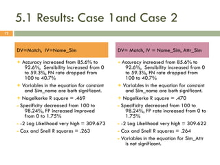
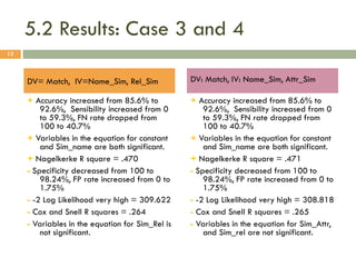
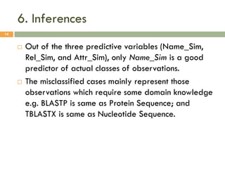
This document describes a study on matching conceptual models by comparing entities across different models. The study represented 20 conceptual models as structured tables with information on each entity's name, attributes, and relationships. It then generated a dataset comparing each pair of entities across models based on name, attribute, and relationship similarity metrics. Binary logistic regression was used to analyze how well each metric predicted if entities actually matched, finding that only name similarity was a significant predictor. The study aims to improve the similarity functions and classification approach to better match conceptual models.

1. 1
MATCHING CONCEPTUAL MODELS
(PART OF THE ‘IBIOSEARCH’ PROJECT)
JUNE 9 2008
Quantitative Methods
Ritu Khare

2. Order of the Presentation
2




Problem and
Background
Research Questions
Initial Dataset
Overall Methodology
Representation of
Dataset A
 Criteria to compare two
entities
 Generation of dataset B
 Multivariate Analysis of
dataset B


Results
Case I
 Case II
 Case III
 Case IV




Inferences
Future Work
References

3. 1. Problem and Background
3

Search Interface is represented as a Conceptual Model
C
A
Search X
A:
B:
Search Y
C:



X
B
The aim is to combine all search interfaces i.e. to
combine several conceptual models.
Hence, matching of models is required.
In this project, focus is on matching of entities.
Y

4. 2. Research Questions
4



Find an Entity Matching Technique(s) to match
entities of two models.
Does this technique (or combination of techniques )
provide a good way to compare two entities?
What other basis of comparison can be used?

5. 3. Initial Dataset A
5


20 Conceptual Models
Expect
Example 1:
Matrix
Domain
DB

Example 2:
BLASTP
Alignments
Accession
No.
Gene
ID
Title
Sequence
Gene Patent
Patent
Sequence
Number
Gene
Name

6. 4. Overall Methodology
6
Conceptual
Models
Representation of Dataset A into
structured tables
Criteria to compare entities from different
models
(Entity Name, Attribute set, Relationship Set)
Generation of Dataset B
Multivariate Analysis of Dataset B
Analysis
Results

7. 4.1 Representation of dataset A
7

Every model is represented as


List of entities
Every Entity in a model is represented as
Entity Name
 List of attributes
 List of relationships


Dataset A has the following columns:
(Model_ID, Entity_name, Attribute_set, Relationship_set)

8. 4.2 Criteria to compare two entities
8


All entities from two different models are compared.
Criteria to compare two entities
Entity Name Similarity
Exact String Matching, Substring Matching
Output: Boolean Variable (True, False)
 Attribute Set Similarity
Jaccard Coefficient
Output: Decimal Number (between 0 and 1)
 Relationship Set Similarity
Jaccard Coefficient
Output: Decimal Number (between 0 and 1)


9. 4.3 Generation of Dataset B
9


Input: 20 Conceptual Models
Algorithm:



Stem Entity Names and Attribute Names (Porter Stemmer)
Compare each pair of Entities from different models based on
the three criteria (Slide 7)
Output: Table (598 records)
Pair#
Name Similarity
Attribute Similarity Relationship Similarity
XYZ
Yes
0.657
0.004

10. 4.4 Multivariate Analysis of dataset B
10


Manually annotate if a pair represents similar entities or not. (“Match”
column)
60 matches and 538 mismatches were found.
Pair#
Name
Sim.
Attribute
Sim.
Relationsh
ip Sim.
XYZ

Match
Yes
Yes
0.657
0.004
Is this a good Classification Model?



Can it correctly identify matching and non-matching pair?
Which technique is suitable to answer these questions?
Binary Logistic Regression

Predictive variables are a combination of continuous and categorical variables.

Name_Sim (Categorical), Attr_Sim (Continuous), Rel_Sim (Continuous)

11. 5. Results
11

Binary Logistic Regression
IV: Name_Sim, Attr_Sim, Rel_Sim
 DV: Match





Case I: IV = Name_Sim
Case 2: IV = Name_Sim, Attr_Sim
Case 3: IV = Name_Sim, Rel_Sim
Case 4: IV = Name_Sim, Attr_Sim, Rel_Sim

12. 5.1 Results: Case 1and Case 2
12
DV=Match, IV=Name_Sim
DV= Match, IV = Name_Sim, Attr_Sim
+ Accuracy increased from 85.6% to
92.6%, Sensibility increased from 0
to 59.3%, FN rate dropped from
100 to 40.7%
+ Variables in the equation for constant
and Sim_name are both significant.
+ Nagelkerke R square = .469
- Specificity decreased from 100 to
98.24%, FP increased improved
from 0 to 1.75%
- -2 Log Likelihood very high = 309.673
- Cox and Snell R squares = .263
+ Accuracy
increased from 85.6% to
92.6%, Sensibility increased from 0
to 59.3%, FN rate dropped from
100 to 40.7%
+ Variables in the equation for constant
and Sim_name are both significant.
+ Nagelkerke R square = .470
- Specificity decreased from 100 to
98.24%, FP rate increased from 0 to
1.75%
- -2 Log Likelihood very high = 309.622
- Cox and Snell R squares = .264
- Variables in the equation for Sim_Attr
is not significant.

13. 5.2 Results: Case 3 and 4
13
DV= Match, IV=Name_Sim, Rel_Sim
DV: Match, IV: Name_Sim, Attr_Sim
+ Accuracy increased from 85.6% to
92.6%, Sensibility increased from 0
to 59.3%, FN rate dropped from
100 to 40.7%
+ Variables in the equation for constant
and Sim_name are both significant.
+ Nagelkerke R square = .470
- Specificity decreased from 100 to
98.24%, FP rate increased from 0 to
1.75%
- -2 Log Likelihood very high = 309.622
- Cox and Snell R squares = .264
- Variables in the equation for Sim_Rel is
not significant.
+ Accuracy increased from 85.6% to
92.6%, Sensibility increased from 0
to 59.3%, FN rate dropped from
100 to 40.7%
+ Variables in the equation for constant
and Sim_name are both significant.
+ Nagelkerke R square = .471
- Specificity decreased from 100 to
98.24%, FP rate increased from 0 to
1.75%
- -2 Log Likelihood very high = 308.818
- Cox and Snell R squares = .265
- Variables in the equation for Sim_Attr,
and Sim_rel are not significant.

14. 6. Inferences
14


Out of the three predictive variables (Name_Sim,
Rel_Sim, and Attr_Sim), only Name_Sim is a good
predictor of actual classes of observations.
The misclassified cases mainly represent those
observations which require some domain knowledge
e.g. BLASTP is same as Protein Sequence; and
TBLASTX is same as Nucleotide Sequence.

15. 7. Future Work
15





Improve Similarity Function
Use of domain dictionaries
Include more number of models
Generate a new classification function
Clustering entities that are found similar

16. References
16




NAR Journal dataset
Porter’s Stemming Algorithm:
http://tartarus.org/~martin/PorterStemmer/
Sharma, S. (1995), Applied Multivariate Techniques,
John Wiley & Sons, Inc. New York, NY, USA.
INFO 692 Lecture Handouts

17. 17
Thank You
Questions, Comments, Ideas…?