1. Bayesian Analysis (2012) 7, Number 4, pp. 771–782
On the Limiting Behavior of the “Probability of
Claiming Superiority” in a Bayesian Context
Morris L. Eaton⇤
, Robb J. Muirhead†
and Adina I. Soaita‡
Abstract. In the context of Bayesian sample size determination in clinical trials,
a quantity of interest is the marginal probability that the posterior probability of
an alternative hypothesis of interest exceeds a specified threshold. This marginal
probability is the same as “average power”; that is, the average of the power func-
tion with respect to the prior distribution when using a test based on a Bayesian
rejection region. We give conditions under which this marginal probability (or av-
erage power) converges to the prior probability of the alternative hypothesis as the
sample size increases. This same large sample behavior also holds for the average
power of a (frequentist) consistent test. We also examine the limiting behavior
of “conditional average power”; that is, power averaged with respect to the prior
distribution conditional on the alternative hypothesis being true.
Keywords: Bayesian design, probability of a successful trial, average power, Bayesian
hypothesis testing, clinical trials, sample size determination
1 Introduction
In a recent paper, Muirhead and Soaita (2012) discuss the problem of sample size
determination (SSD) in a clinical trial setting from a Bayesian viewpoint. They focus
on a criterion for SSD they call the “probability of a successful trial” (PST). (Many
statisticians involved in clinical trials use the informal term “successful trial” to mean
that the trial data supports the hypothesis that the experimental drug is superior to
a control (placebo or an existing drug).) To describe this notion, consider data X(n)
from a parametric model Pn(·|✓), with ✓ an element of a parameter space ⇥. In all
practical situations, both X(n) and ✓ will be elements of subspaces of finite dimensional
Euclidean spaces.
Now, consider a proper prior distribution ⇡ on ⇥ and partition ⇥ into two disjoint
subsets ⇥0 and ⇥1. The inferential interest is in concluding that ✓ 2 ⇥1. Let Qn(·|x(n))
denote the posterior distribution on ⇥ given the sample X(n) = x(n); and let ⌘ 2 (0, 1)
be a pre-specifed threshold value. Muirhead and Soaita (2012) define a “successful trial”
(i.e. a trial where we are able to declare superiority) as one for which
Qn(⇥1|x(n)) ⌘. (1)
At the design stage, the left side of (1) cannot be evaluated, as the sample has not yet
been observed. Thus we consider the set of all samples leading to a successful trial,
⇤School of Statistics, University of Minnesota, Minneapolis, MN, eaton@stat.umn.edu
†Statistical Consultant, Lyme, CT, robb.muirhead@yahoo.com
‡Pfizer Inc, Groton, CT, adina.soaita@pfizer.com
2012 International Society for Bayesian Analysis ba0001

2. 772 “Probability of Claiming Superiority”
namely
E⇤
n = {x(n) : Qn(⇥1|x(n)) ⌘} (2)
and look at the marginal probability (under the model and the prior) of E⇤
n. In other
words, we calculate
(n) = E IE⇤
n
(X(n)) (3)
where the expectation E is under the marginal distribution of X(n) and IE⇤
n
is the
indicator function of the set E⇤
n. Muirhead and Soaita (2012) refer to (n) in (3) as the
“probability of a successful trial” (PST) and discuss its use in Bayesian SSD.
It is reasonable to refer to the set E⇤
n as a “Bayesian rejection region”. We note that
the (classical) power function of the test of H0 : ✓ 2 ⇥0 versus H1 : ✓ 2 ⇥1 based on
E⇤
n is just
n(✓) = E✓{IE⇤
n
(X(n))}, (4)
with expectation taken with respect to the model. Then (n) in (3) is the same as
(n) =
Z
⇥
n(✓)⇡(d✓) = E⇡{ n(✓)}, (5)
with expectation taken with respect to the prior ⇡. The expressions (3) and (5) may help
to explain why there is no consistent terminology in the literature. When the rejection
region of a test is taken to be one that is based on a frequentist (non-Bayesian) con-
struction, (n) has been called “average power”, “predictive power”, and “assurance”
(see Whitehead et al. (2008), O’Hagan et al. (2005)). When it is based on a Bayesian re-
jection region (such as E⇤
n in (2)), (n) has also been called “expected Bayesian power”
(see Spiegelhalter et al. (2004)) and “predictive probability” (see Brutti et al. (2008)).
In what follows, we will generally refer to (n), based on the rejection region E⇤
n, as
either the PST or simply as “average power”.
A goal of this paper is to show that for each ⌘ 2 (0, 1), under conditions specified in
Section 2
lim
n!1
(n) = ⇡(⇥1), (6)
i.e., the average power, as given in (3) and (5), converges to the prior probability that
⇥ 2 ⇥1. This is Theorem 1 in Section 2. Brutti et al. (2008) derive (6) in a very special
case, a single sample from a normal distribution with known variance. The limiting
result in (6) plays an important role in the applied use of (n) in determining a sample
size at the design stage. See Muirhead and Soaita (2012) for illustrative examples and
further discussion.
The result (6) is established under two important assumptions. The first of these is
that
⇡(@⇥1) = 0 (7)
where @⇥1 is the topological boundary of ⇥1. We note that (7) is just the well known
definition of “⇥1 is a ⇡-continuity set” (see Billingsley (1968)). The second assumption
is that the posterior is “⇡-consistent”. This notion, defined carefully in Section 2,
has its origins in a result of Doob (1949). In essence, this result shows that in the

3. M. L. Eaton, R. J. Muirhead and A. I. Soaita 773
case of an i.i.d. sample, there is a set C0 ✓ ⇥ such that ⇡(C0) = 1 and for each
✓0 2 C0, the posterior Qn(·|X(n)) converges weakly to the point mass at ✓0, a.s. P(·|✓0).
(Assumptions, and the nature of P, are detailed in Section 2.) Doob’s theorem is
discussed more completely in the Appendix, where an extension to the two sample
problem is described. A careful statement and illustrative proof of Doob’s theorem can
be found in Ghosh and Ramamoorthi (2003).
In Section 2 we also examine the limiting behavior of “average power given that
✓ 2 ⇥1”, a quantity defined later in (18). The main results here are given in Theo-
rems 2 and 3. Section 3 contains examples, the most important of which concerns the
comparison of two normal means. The paper concludes with a discussion (Section 4).
2 Main Theorems
In this section, notation and assumptions are given, followed by statements and proofs.
First, to formulate our asymptotic result, (6), consider a sequence of random vectors
X(n) = (X1, . . . , Xn), (n 1), with each Xi in R1
. Thus the sample space for X(n) is
Rn
, for n = 1, 2, . . .. The coordinates of X(n) are not assumed here to be independent,
although they will be so in the examples in Section 3.
Let ⇥ be a parameter space which is assumed to be a Polish space. Let Pn(·|✓)
denote the distribution of X(n) on Rn
, n = 1, 2, . . .. We further assume that there is a
probability space (R1
, B1
, P(·|✓)) so that Pn(·|✓) is the projection of P(·|✓) onto Rn
.
That is, if B is a Borel set in Rn
(so B ⇥ R1
⇥ R1
⇥ · · · 2 B1
), then
Pn(B|✓) = P(B ⇥ R1
⇥ R1
⇥ · · · |✓). (8)
For x = (x1, x2, . . .) 2 R1
, let x(n) denote the vector of the first n coordinates of x.
Because the Pn(·|✓)’s are the projections of P(·|✓) onto Rn
, for each integrable f defined
on Rn
, we have
Z
Rn
f(x(n))Pn(dx(n)|✓) =
Z
R1
f(x(n))P(dx|✓) (9)
for each ✓ 2 ⇥.
Next, let ⇡ be a proper prior distribution on ⇥. Given X(n) = x(n) 2 Rn
, let
Qn(·|x(n)) be a version of the posterior distribution of ✓.
Definition 2.1: The sequence of posteriors {Qn(·|x(n))} is consistent at ✓0 2 ⇥ if there
is a set B0 ✓ R1
such that P(B0|✓0) = 1, and for each x 2 B0 and each neighborhood
U of ✓0,
lim
n!1
Qn(U|x(n)) = 1.
Remark 2.1: Because ⇥ is a Polish space, it follows from Remark 1.3.1 in Ghosh and
Ramamoorthi (2003) that {Qn(·|x(n))} is consistent at ✓0 i↵ Qn(·|x(n)) converges weakly
to ✓0
(point mass at ✓0) a.s. P(·|✓0).

4. 774 “Probability of Claiming Superiority”
Definition 2.2: The sequence of posteriors {Qn(·|x(n))} is ⇡-consistent if there is a
set C0 ✓ ⇥ such that ⇡(C0) = 1 and for each ✓0 2 C0, the sequence of posteriors is
consistent at ✓0.
In essence, the theorem of Doob (1949) states that in the i.i.d. case, when both the
sample space and parameter space are Polish spaces, then the sequence of posteriors is
⇡-consistent for each prior ⇡.
We now proceed to formulate Theorem 1 below that will imply equation (6). To this
end, let C be a Borel subset of ⇥. Fix ⌘ 2 (0, 1) and let
En = {x(n) : Qn(C|x(n)) ⌘}. (10)
Note that the dependence of En on the set C is suppressed. Our general result below
is formulated for an arbitrary Borel set C.
With Mn(·) denoting the marginal distribution of X(n) (under the model and the
prior), our main result describes the asymptotic behavior of
(n) = Mn(En). (11)
Obviously, for each Borel subset B of Rn
,
Mn(B) =
Z
⇥
Z
Rn
IB(x(n))Pn(dx(n)|✓)⇡(d✓)
=
Z
⇥
Z
R1
IB(x(n))P(dx|✓)⇡(d✓). (12)
Finally, we recall some standard topological notation. For a subset D ✓ ⇥, D is
the interior of D, ¯D is the closure of D, Dc
is the complement of D and @D is the
boundary of D. Note that the boundary of D is equal to the boundary of Dc
.
Theorem 1: Suppose that {Qn(·|x(n))} is ⇡-consistent and that ⇡(@C) = 0. Then
lim
n!1
(n) = ⇡(C), (13)
where (n) is given by (11).
Proof: By assumption, there is a set C0 ✓ ⇥ with ⇡(C0) = 1 and such that the sequence
of posteriors is consistent at ✓0 for each ✓0 2 C0. Because ⇡(@C) = 0, we can write
(n) =
Z
C
Z
R1
IEn (x(n))P(dx|✓)⇡(d✓) +
Z
(Cc)
Z
R1
IEn (x(n))P(dx|✓)⇡(d✓)
= 1(n) + 2(n). (14)
To analyze 1(n), fix ✓0 2 C C0. Since C is a neighborhood of ✓0 and the posterior
is consistent at ✓0, it follows that
lim
n!1
Qn(C|x(n)) = 1 a.s. P(·|✓0).

5. M. L. Eaton, R. J. Muirhead and A. I. Soaita 775
Thus
lim
n!1
IEn
(x(n)) = 1 a.s. P(·|✓0).
Since ⇡(C0) = 1, we can apply the dominated convergence theorem to see that
lim
n!1
1(n) =
Z
C0
⇡(d✓) = ⇡(C0
).
But ⇡(@C) = 0, so ⇡(C) = ⇡(C0
).
A similar argument shows that
lim
n!1
2(n) = 0.
This completes the proof.
The application of Theorem 1 to the problem described in Section 1 requires the
verification of two main assumptions. We need to show that @⇥1 has prior probability
zero and that the posterior distribution is ⇡-consistent. In the i.i.d. case, the theorem
of Doob (1949) applies to show that ⇡-consistency holds. The boundary condition on
⇥1 needs to be checked in each application.
Remark 2.2: Theorem 1 above is proved under two assumptions, namely that the
posterior is ⇡-consistent and that ⇡(@C) = 0. Modifications of these are possible while
maintaining the validity of (13). For example, if we assume that (i) C is open,
(ii) Qn(@C|x(n)) ! 1 a.s. P(·|✓) for all ✓ 2 @C,
and (iii) ⇡-consistency, then (13) holds. A simple modification of the proof of Theorem 1
establishes this assertion.
An example of this is the following. Assume X1, . . . , Xn are i.i.d. N(✓, 1), ⇥ = R1
,
⇥0 = ( 1, 0], ⇥1 = (0, 1), so @⇥1 = {0}. Consider the prior ⇡ = 1
2 ⇡0 + 1
2 ⇡1, where
⇡0 is a point mass at 0 and ⇡1 is N(0, 1). With C = ⇥1, ⇡(@C) = 1
2 , but a routine
calculation shows
Qn({0}|x(n)) ! 1 a.s. P(·|0)
and we have
(n) !
1
4
= ⇡(⇥1).
A frequentist version of Theorem 1 is easy to formulate. Suppose that Rn is the
rejection region of a test of ⇥0 versus ⇥1 and let n be the corresponding test function
(the indicator function of Rn). The power function of the test n is just
n(✓) = E✓( n),
with expectation taken with respect to the model. The frequentist testing procedure
defined by n is asymptotically consistent for testing ⇥0 versus ⇥1 if, as n ! 1, n(✓)

6. 776 “Probability of Claiming Superiority”
converges to 1 on the interior of ⇥1 and converges to 0 on the interior of ⇥0. Now, if ⇡
is a proper prior distribution on ⇥ such that ⇡(@⇥1) = 0, it is routine to show that
lim
n!1
Z
⇥
n(✓)⇡(d⇥) = ⇡(⇥1)
for asymptotically consistent tests. This of course is a frequentist analog of Theorem 1.
Taking Rn = E⇤
n (as defined in (2)) establishes the Bayesian-frequentist connection.
Because of the limit result (6), and because (n) is increasing in n in their examples,
Muirhead and Soaita (2012) suggested that it may be preferable, when choosing a sample
size, to focus attention on a “normalized index” ⇤
(n) given by
⇤
(n) =
(n)
⇡(⇥1)
, (15)
for which
lim
n!1
⇤
(n) = 1, (16)
so that ⇤
(n) represents the proportion of the maximum value of the PST (average
power) explained by the sample size n. We now look at an alternative proposal.
Recall from (5) that the average power (n) may be written as
(n) =
Z
⇥
n(✓)⇡(d✓), (17)
where n(✓) is the (classical) power function of the test with rejection region E⇤
n given
by (2). A referee suggested that since our hope is to be able to conclude that ✓ 2 ⇥1, it
would also be of interest to consider “average Bayesian power given that ✓ 2 ⇥1”; that
is, to investigate the quantity ˜(n) given by
˜(n) =
1
⇡(⇥1)
Z
⇥1
n(✓)⇡(d✓). (18)
Of course, ˜(n) is the average power with respect to the prior distribution conditional
on “✓ 2 ⇥1”. That is, let
˜⇡(A) =
⇡(A ⇥1)
⇡(⇥1)
, A ✓ ⇥. (19)
Then ˜⇡ is the conditional prior obtained from ⇡ given that ✓ 2 ⇥1. It is clear that
˜(n) =
Z
⇥
n(✓)˜⇡(d✓). (20)
It is now natural to ask how ˜(n) behaves as n ! 1. An obvious analog to Theorem 1
answers this question.

7. M. L. Eaton, R. J. Muirhead and A. I. Soaita 777
Theorem 2: Suppose that {Qn(·|x(n))} is ⇡-consistent and that ⇡(@⇥1) = 0. Then
lim
n!1
˜(n) = 1.
Proof: The proof is a minor modification of the proof of Theorem 1. The details are
omitted.
A useful alternative form of Theorem 2 is available when the alternative ⇥1 is actu-
ally an open set, as in the case of many interesting examples.
Theorem 3: Suppose that {Qn(·|x(n))} is ⇡-consistent and that ⇥1 is a non-empty
open set. Then
lim
n!1
˜(n) = 1.
Proof: Since {Qn(·|x(n))} is ⇡-consistent, the test with rejection region E⇤
n is (frequen-
tist) asymptotically consistent. The openness of ⇥1 implies that n(✓) ! 1 for each
✓ 2 ⇥1. The bounded convergence theorem gives the desired conclusion.
3 Examples
The simplest examples of Theorem 1 concern i.i.d. samples, since Doob’s theorem
implies ⇡-consistency. For example, with data X(n) = (X1, . . . , Xn) where X1, . . . , Xn
are i.i.d. N(µ, 2
), consider testing ⇥0 = {µ, 2
| µ  0} versus ⇥1 = {µ, 2
| µ > 0}.
For any prior ⇡ on ⇥ = ⇥0 [ ⇥1 that is absolutely continuous with respect to Lebesgue
measure dµd , we have ⇡(@⇥1) = 0, so Theorem 1 implies that (n) converges to ⇡(⇥1).
The main example of this section involves data from two independent normal sam-
ples.
Example 3.1: Let X1, . . . , Xm and Y1, . . . , Yn be independent, with the X’s i.i.d.
N(µ1, 2
) and the Y ’s i.i.d. N(µ2, 2
). We consider the case where the three parameters
are unknown (the case of known 2
is a little easier). In this example,
⇥ = {µ1, µ2, 2
| µi 2 R1
, i = 1, 2 and > 0},
⇥0 = {µ1, µ2, 2
| µ1  µ2}, and ⇥1 = {µ1, µ2, 2
| µ1 > µ2}.
Clearly @⇥1 = {µ1, µ2, 2
| µ1 = µ2} and @⇥1 has Lebesgue measure zero when ⇥ is
considered a subset of R3
.
Let ⇡ be a prior on ⇥ that is absolutely continuous with respect to Lebesgue measure.
Given this prior for ✓ = (µ1, µ2, ), let Qm,n(d✓|X(m), Y(n)) denote the posterior. With
p = min{m, n}, the argument in the Appendix shows that when p ! 1, the posterior
is ⇡-consistent. Since ⇡(@⇥1) = 0, Theorem 1 implies that
lim
p!1
(p) = ⇡(⇥1). (21)
The use of this result in determining sample sizes is discussed in Muirhead and Soaita
(2012).

8. 778 “Probability of Claiming Superiority”
Example 3.2: This example is intended to illustrate the two measures ⇤
(n) given
by (15) and ˜(n) given by (18). It is based on Example 3.1.1 in Muirhead and Soaita
(2012) where the subjects in the clinical trial have “Restless Legs Syndrome”. Let U
be the di↵erence between the disease score sample means of two goups (experimental
drug and placebo), with equal sample sizes n1 in each group, so that the total sample
size is n = 2n1. Under standard normality assumptions, U ⇠ N( , 4 2
/n), where 2
is the common variance in each group, and where > 0 favors the experimental drug.
The variance 2
is assumed known (from an earlier study), with = 8. For a 1-sided
0.025-level z-test to have 80% power at the “clinically meaningful di↵erence”of 4 (drug
versus placebo), 64 subjects in each group are required, for a total sample size of 128.
In one of the settings in Muirhead and Soaita (2012), the prior distribution for the
treatment e↵ect is N( , 64), and the threshold in (1) used to define a “successful
trial” is ⌘ = 0.975. Graphs of the normalized index ⇤
(n) versus n are given in Figure 1
of Muirhead and Soaita (2012) for various values of the prior mean . It is pointed out
(for example) that, when = 4 (the “clinically meaningful” e↵ect size), ⇤
(100) = 0.79,
and there is not much to be gained (in terms of the PST (average power)) by taking
a larger total sample size than n = 100. What is interesting is that, for the range of
’s considered, there turns out to be no discernible di↵erence between the graphs of
⇤
(n) versus n and ˜(n) versus n. The primary reason for this here is the fact that the
threshold ⌘ = 0.975 is set very high, as it would need to be for regulatory drug approval.
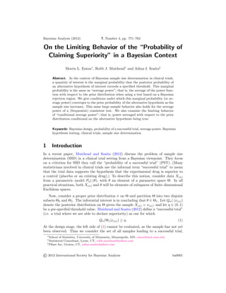
A lower value of the the threshold ⌘ would be appropriate in exploratory and early
phase trials, and this is where we see a di↵erence between ⇤
(n) and ˜(n). Figure 1
gives the graphs of both ⇤
(n) and ˜(n) when ⌘ = 0.8 (and = 4). (Both functions
converge to one as n ! 1.) As is to be expected, ˜(n) < ⇤
(n) for each n. For
example, if the total sample size is n = 20, we have ⇤
(20) = 0.82 and ˜(20) = 0.79.
For further discussion, see Section 4.
4 Discussion and summary
We began this paper with a focus on (unconditional) average power given in (3) and
(5), namely
(n) = P(X(n) 2 E⇤
n) = P(reject H0),
where the set E⇤
n given in (2) is a Bayesian rejection region, and where the probability
involved is computed using the marginal distribution of X(n). We established conditions
(Theorem 1) under which, as n ! 1,
(n) ! ⇡(⇥1) (22)
the prior probability of H1. (Under these conditions, the “normalized average power”
⇤
(n) given by (15) converges to one.) We also noted that the limiting result (22) also
holds if E⇤
n is replaced by the rejection region of a test that is asymptotically consistent
(in the usual classical sense).
We further considered the “conditional power” ˜(n) given by (18), and established

9. M. L. Eaton, R. J. Muirhead and A. I. Soaita 779
0 10 20 30 40 50 60 70 80 90 100 110 120
0.4
0.5
0.6
0.7
0.8
0.9
1
Total sample size n
Functionvalue
⇤
(n)
˜(n)
Figure 1: Graphs of ⇤
(n) and ˜(n) when the threshold is ⌘=0.8 (and =4).
conditions (Theorems 2 and 3) under which, as n ! 1,
˜(n) ! 1.
The use of the two quantities ⇤
(n) and ˜(n) in a sample sizing context was illustrated
in Example 3.2.
The quantities , ⇤
, and ˜ are, of course, related. We now detail this, suppressing
the dependence on n. By definition, ⇤
= /⇡(⇥1). Conditioning on whether H0 or
H1 is true gives
= P(reject H0|H1 true)⇡(⇥1) + P(reject H0|H0 true)⇡(⇥0). (23)
Rejecting H0 when it is true represents a false positive (FP), and (23) may be written
= ˜ · ⇡(⇥1) + P(FP)⇡(⇥0)
so that
⇤
= ˜ + P(FP)
⇡(⇥0)
⇡(⇥1)
. (24)
As n ! 1 (and for any fixed ⌘ 2 (0, 1)),
⇤
! 1, ˜ ! 1, and P(FP) ! 0.
Remarks:

10. 780 “Probability of Claiming Superiority”
(a) We noted in Example 3.2 that ˜ < ⇤
. Equation (24) shows that ⇤
is “inflated” by
the probability of a false positive. This latter probability decreases as the threshold
⌘ increases. (We noted in Example 3.2 that there was virtually no di↵erence, for
any n, between ⇤
and ˜ when ⌘ = 0.975, a high threshold. As ⌘ is decreased, a
di↵erence appears in the graphs; this di↵erence, of course, decreases as n increases.)
(b) In a sample sizing problem, it is natural to ask: If the alternative is true, what is
the probability that (using the Bayesian rejection region (2)) we conclude that this
is so. This probability is the “conditional power” ˜(n) (see (18) and (20)). We
would then select a sample size n⇤
as the smallest value of n such that ˜(n) ,
where 2 (0, 1) is a pre-specified number. In other words, n⇤
is the smallest value
of n such that the conditional probability of deciding in favor of the alternative,
given the alternative is true, is at least . In our view, the use of ˜ (rather than
or ⇤
) appears to be the most plausible of the three “average power functions” in
explaining the application to sample sizing.
(c) Finally, there may be a technical advantage to preferring ˜ in some situations.
Theorem 3 shows that the conditional power converges to 1, even when the boundary
@⇥1 of ⇥1 has positive probability under the prior.
References
Billingsley, P. (1968). Convergence of Probability Measures. New York: Wiley. 772
Blackwell, D. and Dubins, L. (1962). “Merging of opinions with increasing information.”
Annals of Mathematical Statistics, 33: 882–886. 782
Brutti, P., De Santis, F., and Gubiotti, S. (2008). “Robust Bayesian sample size deter-
mination in clinical trials.” Statistics in Medicine, 27: 2290–2306. 772
Doob, J. L. (1949). “Application of the theory of martingales.” In Le Calcul des
Probabilites et ses Applications, 23–27. Centre National de la Recherche Scientifique,
Paris. Colloques Internationalaux du Centre National de le Recherche Scientifique,
no 13. 772, 774, 775
Ghosh, J. K. and Ramamoorthi, R. V. (2003). Bayesian Nonparametrics. New York:
Springer Verlag. 773, 781
Muirhead, R. J. and Soaita, A. I. (2012). “On an approach to Bayesian sample sizing
in clinical trials.” In Jones, G. and Shen, X. (eds.), Multivariate Statistics in Modern
Statistical Analysis: A Festschrift in honor of Morris L. Eaton. Institute of Mathemat-
ical Statistics, Beachwood, Ohio. To appear. Available online at arXiv:1204.4460v1.
771, 772, 776, 777, 778
O’Hagan, A., Steven, J. W., and Campbell, M. J. (2005). “Assurance in clinical trial
design.” Pharmaceutical Statistics, 4: 187–201. 772

11. M. L. Eaton, R. J. Muirhead and A. I. Soaita 781
Spiegelhalter, D. J., Abrams, K. R., and Myles, J. P. (2004). Bayesian Approaches to
Clinical Trials and Health Care Evaluation. New York: Wiley. 772
Whitehead, J., Valdes-Marquez, E., Johnson, P., and Graham, G. (2008). “Bayesian
sample size for exploratory clinical trials incorporating historical data.” Statistics in
Medicine, 27: 2307–2327. 772
Appendix
The purpose of this appendix is to argue that in the two sample case of Example 3.1,
the posterior is ⇡-consistent. Of course, assumptions are needed to make this claim
correct. These will be detailed in the discussion below.
Consider sequences X1, X2, . . . and Y1, Y2, . . . of real valued random variables and
assume that the X’s are i.i.d. P1(·|✓), the Y ’s are i.i.d. P2(·|✓), and the X’s and Y ’s
are independent. The parameter ✓ is an element of a Polish space ⇥. Given a positive
integer k, let Z(k) = (Z1, . . . , Zk) where Zi = (Xi, Yi), i = 1, 2, . . . . Then the Zi’s are
i.i.d. on R2
with distribution P3(·|✓) ⌘ P1(·|✓)⇥P2(·|✓). Let Fk be the -field generated
by Z(k) and let ⇡ be a prior distribution on ⇥. Under the assumption that the map
✓ ! P3(·|✓) is 1 1, Doob’s Theorem (see Theorem 1.3.2 on page 22 of Ghosh and
Ramamoorthi (2003)) implies that the posterior distribution Qk(·|Z(k)) is ⇡-consistent.
Of course, in standard -field notation,
Qk(·|Z(k)) = Qk(·|Fk).
A basic step in the proof of Doob’s Theorem uses the Martingale Convergence Theorem
to conclude that for each Borel set C ✓ ⇥,
lim
k!1
Qk(C|Z(k)) = lim
k!1
E(IC|Fk) = E(IC|F1),
where F1 is the limit of increasing -fields Fk. One then shows there is a set ⇥0 ✓ ⇥
such that ⇡(⇥0) = 1 and for ✓ 2 ⇥0 C,
E(IC|F1) = 1 a.e. P1
(·|✓), (25)
where P1
(·|✓) is the infinite product measure P3(·|✓) ⇥ P3(·|✓) ⇥ · · · . That this estab-
lishes the ⇡-consistency is argued on pages 23-24 of Ghosh and Ramamoorthi (2003).
To apply the above to the two sample problem of Example 3.1, consider sequences
m1, m2, . . . and n1, n2, . . . of non-decreasing positive integers both converging to infinity.
Let (X1, . . . , Xmp
) = X(mp) and (Y1, . . . , Ynp
) = Y(np) be a sample of X’s and Y ’s.
Let Gp be the -field generated by {X(mp), Y(np)} and let Q⇤
p(·|Gp) be a version of the
conditional distribution of ✓ given {X(mp), Y(np)}. Thus, for a Borel set C ✓ ⇥,
Q⇤
p(C|Gp) = E(IC|Gp)
for p = 1, 2, . . . . With k = min{np, mp}, note that
Fk ✓ Gp ✓ F1.

12. 782 “Probability of Claiming Superiority”
Since Fk converges to F1, it follows that Gp converges to F1. This implies (see Theorem
2 in Blackwell and Dubins (1962)) that
lim
p!1
E(IC|Gp) = E(IC|F1).
However, this is characterized by (25) which in turn shows that Q⇤
p(·|Gp) is a ⇡-consistent
sequence of posteriors.
It is clear that the above argument can be extended to the r-sample case to establish
the ⇡-consistency of a posterior. Note that ⇡-consistency can fail rather dramatically
when observations are not independent. For example, consider X(n) 2 Rn
which is
Nn(✓, ⌃0), where the vector of means ✓ 2 Rn
has all its coordinates equal to an unknown
parameter µ, and where the n ⇥ n covariance matrix ⌃0 has diagonal elements equal to
1 and o↵-diagonal elements equal to a known value ⇢ 2 (0, 1). If we take a N(0, 1) prior
for µ, the posterior can be calculated explicitly and is not ⇡-consistent.
Acknowledgments
The authors would like to thank a referee for many thoughtful and insightful comments.