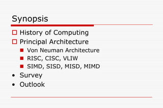
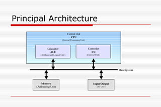
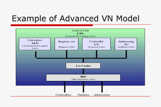
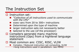
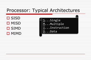
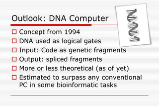
This document discusses processor architectures and their history. It begins with an overview of the history of computing from early switches to modern microprocessors. It then describes the principal Von Neumann architecture and variations like RISD, CISC, and VLIW. It also covers parallel architectures like SIMD, SISD, MISD, and MIMD. The document provides examples of different processor types and looks at potential future architectures like DNA and quantum computing.

1. Processor Architectures
Lorenz Sauer
2003/04

2. Synopsis
 History of Computing
 Principal Architecture
 Von Neuman Architecture
 RISC, CISC, VLIW
 SIMD, SISD, MISD, MIMD
• Survey
• Outlook

3. History of Computing
 1st Switches
 2nd Binary Theory (comprehensive)
 Implemented as:
 Tubes
 Transistor
 BiPolar
 FET (especially MOSFET)
 Future (DNA,...)

4. Hardware-means to the end...
 Tube Technology
 huge, high power dissipation, very slow
 Transistor
 First models: huge
 Minaturization: rapidly
 BiPolar: fast, decent power dissipation
 FET: decent speed, low power dissipation,
extreme Intregration Density is possible

5. Computing Timetable
 1949 John von Neumann
 1970s first microprocessor machines
 1980s IBM PC settling in industry
 1990s large-scale mainframes
 2000s GRID, interconnected computing
 >2000

6. History: VisiCalc the Killer App
 1979: First released with Apple II
 1981: Ported to IBM PCs
 Convinces the „industry„ of IBM PCs
 New mainstream market born
 Still executable
 27.520bytes of
Spreadsheetness

7. Principal Architecture: Basics
 Processor or Central Processing Unit
 CPU is the heart of a computer
 Execute programs stored in main memory
 Instructions are processed sequentially:
 fetched, examined and executed
 Church–Turing thesis
 The CPU is composed of:
 Control Unit
 Arithmetic logic unit (ALU)
 Registers

8. Principal Architecture
Central Unit
CPU
(Central Processing Unit)
Calculator Controller
ALU CU
(Arithmetical Logical Unit) (Control Unit)
Bus System
Memory Input/Output
(Addressing Unit) (IO Unit)

9. Instruction Execution
 Pure VN(Von Neuman)-Execution Model
 Nowadays few computers employ pure von
Neumann architecture
 No Check for Interrupts
 Pure VN computers spend a lot of time
moving data from and to memory
 So called “Neumann bottleneck“

10. Instruction Execution
 Advanced VN Model(s)
 Interrupt built in
 Bus Architecture extended over several
busses (different stepping possible)
 Pipelining
 Caching
 Co-Processor (Math, DSP,..)
 Parallelization of Units

11. Example of Advanced VN Model
Central Unit
CPU
(Cent ral P rocessing Unit )
Calculator
Register set Controller Addressing
ALU AU
CU
(Arit hmet ical Logical
(Regist er File) (Cont rol Unit ) (Address Unit )
Unit )
L1-Cache
BIU
(Bus Int erface Unit )
Controlbus Databus Addressbus

12. The Instruction Set
 Instruction set:
 “Collection of all instructions used to communicate
with the CPU“
 sizes vary from 20 to 300+ instructions
 Determined upon the type of machine
 larger instruction sets not necessarily better
 tailored to the use (of the processor)
 Compilers generate many machine
instructions (Ops) from a highlevel language
statement
 Most common are: CISC, RISC, VLIW
 Complex / Reduced instruction set computing, VLIW
~long instructions used in parallelism: see MIMD

13. Processor: Typical Architectures
 SISD
S...Single
 MISD M...Multiple
 SIMD I...Instruction
D...Data
 MIMD

14. SISD
 Single Instruction Single Data
 Almost any conventional PC is SISD
 VN-model is a pure SISD

15. MISD
 Multiple Instruction Single Data
 No commercial success
 Example: Systolic Processor

16. SIMD
 Single Instruction Multiple Data
 Executes operations in parallel
 Example: Vector computer aka Array
computer (~history of supercomputers)
 Nowadays as SIMD extensions
 Speeds up certain applications: chiefly
multimedia (~rich in single precision
floating point data)

17. MIMD
 Multiple Instruction Multiple Data
 Parallel architecture
 Many functional units
 Performs different operations on
seperate data
 Example: Multiprocessor,
interconnected workstations

18. Other: Vector-, Array-Processor
 Common in supercomputers till 1980s
 performs operations in parallel
 Copes well with large data chunks
 Bad under general purpose conditions
 Nowadays in PC-CPUs as SIMD

19. Other: Artificial Neural Processor
 Employed for pattern recognition
 Artificial Neural Network(ANN) model
 mutually linked, homogeneous
processing units
 Units perform basic ANN operations:
 Threshold calculation
 Weighting
 Addition,....

20. Other: Parallel Reduction Machine
 Simplification of expressions
 Expressions reshaped into smaller,
partial ones
 Obtained through recursion of partial
expressions
 Performs reduction programs
 String reduction vs. Graph reduction
machines

21. Other: Systolic Processor
 Array of Processing units (Cells)
 Single cell trivial
 Relay data via n - I/O
 Structure: Rectangular, Hexagonal or
triangular
 Elements process same calculation
 Edge cells are the main I/O

22. Other: Fuzzy Processor
 Based on fuzzy logic
 many-valued logic or probabilistic logic
 approximate values rather than fixed (0|1)
 “set of approximate rules”-logic:
 IF variable IS ~property THEN response 1
 IF variable IS >>property THEN response 2
 Examples:
 Washing maschines,Auto focus,...

23. Other: Digital Signal Processor
 Used for very specific tasks
 Implements algorithms in Hardware
 Very fast at specific tasks
 Useless for general purpose programs
 Sufficient for some applications
 Can lower overall costs

24. Survey: GRID Computing
 Used in scenarios to big for single
supercomputers
 Heterogenous structure
 Heterogenous computer-hardware / software and
structure scattered around the globe
 Common middleware necessary
 E.g. Globus Toolkit
 2 Types, determined by their use:
 Computation Grids
 Data Grids
 Examples:
 SETI Project, @Folding: Protein folding...

25. Outlook
 Processor Optimization
 DNA Computer
 Quantum Computer

26. Outlook: Processor Optimization
 Clock Speeds
 Minaturization
 Improved & extended architecture
 Compilers (good at trvial tasks, fail at
more complicated and parallel tasks)
 Non-trivial to determine the use of
instruction extensions
 Most unit extensions are not used

27. Outlook: DNA Computer
 Concept from 1994
 DNA used as logical gates
 Input: Code as genetic fragments
 Output: spliced fragments
 More or less theoretical (as of yet)
 Estimated to surpass any conventional
PC in some bioinformatic tasks

28. Outlook: Quantum Computer
 1981: Quantum computer theory
 Bits vs QBits
 Difficult to generate and maintain,
due to outside effects
 8 bit Computer is in 1 state of 256
 8 Qbit Computer is in n state(s) of 256
 Superposition of states
 Quantum parallelism
 All values exist; a single value is determined at the time
of measurement
 10Qbit computer could surpass a supercomputer
 Problems of error correction and calculation reliability