The document discusses Gibbs flow transport for Bayesian inference, outlining the challenges of obtaining consistent estimators for target distributions and highlighting issues with traditional Markov Chain Monte Carlo methods. It introduces concepts such as annealed importance sampling and the Jarzynski nonequilibrium equality, while also exploring optimal dynamics to enhance estimator performance. Finally, it touches on the dynamics governed by the Liouville equation and the requirements for solving transport problems effectively.

1. Gibbs flow transport for Bayesian inference
Jeremy Heng,
Department of Statistics, Harvard University
Joint work with Arnaud Doucet (Oxford) & Yvo Pokern (UCL)
Computational Statistics and Molecular Simulation:
A Practical Cross-Fertilization
Casa Matem´atica Oaxaca (CMO)
13 November 2018
Jeremy Heng Flow transport 1/ 24

2. Problem specification
• Target distribution on Rd
π(dx) =
γ(x) dx
Z
where γ : Rd
→ R+ can be evaluated pointwise and
Z =
Rd
γ(x) dx
is unknown
Jeremy Heng Flow transport 2/ 24

3. Problem specification
• Target distribution on Rd
π(dx) =
γ(x) dx
Z
where γ : Rd
→ R+ can be evaluated pointwise and
Z =
Rd
γ(x) dx
is unknown
• Problem 1: Obtain consistent estimator of π(ϕ) := Rd ϕ(x) π(dx)
Jeremy Heng Flow transport 2/ 24

4. Problem specification
• Target distribution on Rd
π(dx) =
γ(x) dx
Z
where γ : Rd
→ R+ can be evaluated pointwise and
Z =
Rd
γ(x) dx
is unknown
• Problem 1: Obtain consistent estimator of π(ϕ) := Rd ϕ(x) π(dx)
• Problem 2: Obtain unbiased and consistent estimator of Z
Jeremy Heng Flow transport 2/ 24

5. Motivation: Bayesian computation
• Prior distribution π0 on unknown parameters of a model
Jeremy Heng Flow transport 3/ 24

6. Motivation: Bayesian computation
• Prior distribution π0 on unknown parameters of a model
• Likelihood function L : Rd
→ R+ of data y
Jeremy Heng Flow transport 3/ 24

7. Motivation: Bayesian computation
• Prior distribution π0 on unknown parameters of a model
• Likelihood function L : Rd
→ R+ of data y
• Bayes update gives posterior distribution on Rd
π(dx) =
π0(x)L(x) dx
Z
,
where Z = Rd π0(x)L(x) dx is the marginal likelihood of y
Jeremy Heng Flow transport 3/ 24

8. Motivation: Bayesian computation
• Prior distribution π0 on unknown parameters of a model
• Likelihood function L : Rd
→ R+ of data y
• Bayes update gives posterior distribution on Rd
π(dx) =
π0(x)L(x) dx
Z
,
where Z = Rd π0(x)L(x) dx is the marginal likelihood of y
• π(ϕ) and Z are typically intractable
Jeremy Heng Flow transport 3/ 24

9. Monte Carlo methods
• Typically sampling from π is intractable, so we rely on Markov
chain Monte Carlo (MCMC) methods
Jeremy Heng Flow transport 4/ 24

10. Monte Carlo methods
• Typically sampling from π is intractable, so we rely on Markov
chain Monte Carlo (MCMC) methods
• MCMC constructs a π-invariant Markov kernel
K : Rd
× B(Rd
) → [0, 1]
Jeremy Heng Flow transport 4/ 24

11. Monte Carlo methods
• Typically sampling from π is intractable, so we rely on Markov
chain Monte Carlo (MCMC) methods
• MCMC constructs a π-invariant Markov kernel
K : Rd
× B(Rd
) → [0, 1]
• Sample X0 ∼ π0 and iterate Xn ∼ K(Xn−1, ·) until convergence
Jeremy Heng Flow transport 4/ 24

12. Monte Carlo methods
• Typically sampling from π is intractable, so we rely on Markov
chain Monte Carlo (MCMC) methods
• MCMC constructs a π-invariant Markov kernel
K : Rd
× B(Rd
) → [0, 1]
• Sample X0 ∼ π0 and iterate Xn ∼ K(Xn−1, ·) until convergence
• MCMC can fail in practice, for e.g. when π is highly multi-modal
Jeremy Heng Flow transport 4/ 24

13. Annealed importance sampling
• If π0 and π are distant,
Jeremy Heng Flow transport 5/ 24

14. Annealed importance sampling
• If π0 and π are distant, define bridges
πλm
(dx) =
π0(x)L(x)λm
dx
Z(λm)
,
with 0 = λ0 < λ1 < . . . < λM = 1 so
that π1 = π
Jeremy Heng Flow transport 5/ 24

15. Annealed importance sampling
• If π0 and π are distant, define bridges
πλm
(dx) =
π0(x)L(x)λm
dx
Z(λm)
,
with 0 = λ0 < λ1 < . . . < λM = 1 so
that π1 = π
• Initialize X0 ∼ π0 and move Xm ∼ Km(Xm−1, ·) for m = 1, . . . , M,
where Km is πλm -invariant
Jeremy Heng Flow transport 5/ 24

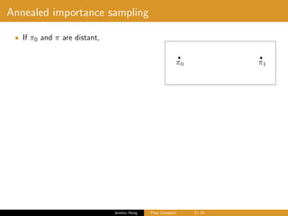
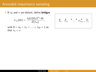
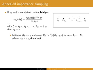
16. Annealed importance sampling
• If π0 and π are distant, define bridges
πλm
(dx) =
π0(x)L(x)λm
dx
Z(λm)
,
with 0 = λ0 < λ1 < . . . < λM = 1 so
that π1 = π
• Initialize X0 ∼ π0 and move Xm ∼ Km(Xm−1, ·) for m = 1, . . . , M,
where Km is πλm -invariant
• Annealed importance sampling constructs w : (Rd
)M+1
→ R+ so
that
π(ϕ) =
E [ϕ(XM )w(X0:M )]
E [w(X0:M )]
, Z = E [w(X0:M )]
Jeremy Heng Flow transport 5/ 24

17. Annealed importance sampling
• If π0 and π are distant, define bridges
πλm
(dx) =
π0(x)L(x)λm
dx
Z(λm)
,
with 0 = λ0 < λ1 < . . . < λM = 1 so
that π1 = π
• Initialize X0 ∼ π0 and move Xm ∼ Km(Xm−1, ·) for m = 1, . . . , M,
where Km is πλm -invariant
• Annealed importance sampling constructs w : (Rd
)M+1
→ R+ so
that
π(ϕ) =
E [ϕ(XM )w(X0:M )]
E [w(X0:M )]
, Z = E [w(X0:M )]
• AIS (Neal, 2001) and SMC samplers (Del Moral et al., 2006) are
considered state-of-the-art in statistics and machine learning
Jeremy Heng Flow transport 5/ 24

18. Jarzynski nonequilibrium equality
• Consider M → ∞,
Jeremy Heng Flow transport 6/ 24

19. Jarzynski nonequilibrium equality
• Consider M → ∞, i.e. define the curve
of distribution {πt}t∈[0,1]
Jeremy Heng Flow transport 6/ 24

20. Jarzynski nonequilibrium equality
• Consider M → ∞, i.e. define the curve
of distribution {πt}t∈[0,1]
πt(dx) =
π0(x)L(x)λ(t)
dx
Z(t)
,
where λ : [0, 1] → [0, 1] is a strictly
increasing C1
function
Jeremy Heng Flow transport 6/ 24

21. Jarzynski nonequilibrium equality
• Consider M → ∞, i.e. define the curve
of distribution {πt}t∈[0,1]
πt(dx) =
π0(x)L(x)λ(t)
dx
Z(t)
,
where λ : [0, 1] → [0, 1] is a strictly
increasing C1
function
• Initialize X0 ∼ π0 and run time-inhomogenous Langevin dynamics
dXt =
1
2
log πt(Xt)dt + dWt, t ∈ [0, 1]
Jeremy Heng Flow transport 6/ 24

22. Jarzynski nonequilibrium equality
• Consider M → ∞, i.e. define the curve
of distribution {πt}t∈[0,1]
πt(dx) =
π0(x)L(x)λ(t)
dx
Z(t)
,
where λ : [0, 1] → [0, 1] is a strictly
increasing C1
function
• Initialize X0 ∼ π0 and run time-inhomogenous Langevin dynamics
dXt =
1
2
log πt(Xt)dt + dWt, t ∈ [0, 1]
• Jarzynski equality (Jarzynski, 1997; Crooks, 1998) constructs
w : C([0, 1], Rd
) → R+ so that
π(ϕ) =
E ϕ(X1)w(X[0,1])
E w(X[0,1])
, Z = E w(X[0,1])
Jeremy Heng Flow transport 6/ 24

23. Jarzynski nonequilibrium equality
• Consider M → ∞, i.e. define the curve
of distribution {πt}t∈[0,1]
πt(dx) =
π0(x)L(x)λ(t)
dx
Z(t)
,
where λ : [0, 1] → [0, 1] is a strictly
increasing C1
function
• Initialize X0 ∼ π0 and run time-inhomogenous Langevin dynamics
dXt =
1
2
log πt(Xt)dt + dWt, t ∈ [0, 1]
• Jarzynski equality (Jarzynski, 1997; Crooks, 1998) constructs
w : C([0, 1], Rd
) → R+ so that
π(ϕ) =
E ϕ(X1)w(X[0,1])
E w(X[0,1])
, Z = E w(X[0,1])
• To what extent is this state-of-the-art in molecular dynamics?
Jeremy Heng Flow transport 6/ 24

24. Optimal dynamics
• Dynamical lag Law(Xt) − πt impacts variance of estimators
Jeremy Heng Flow transport 7/ 24

25. Optimal dynamics
• Dynamical lag Law(Xt) − πt impacts variance of estimators
• Vaikuntanathan & Jarzynski (2011) considered adding drift
f : [0, 1] × Rd
→ Rd
to reduce lag
dXt = f (t, Xt)dt +
1
2
log πt(Xt)dt + dWt, t ∈ [0, 1], X0 ∼ π0
Jeremy Heng Flow transport 7/ 24

26. Optimal dynamics
• Dynamical lag Law(Xt) − πt impacts variance of estimators
• Vaikuntanathan & Jarzynski (2011) considered adding drift
f : [0, 1] × Rd
→ Rd
to reduce lag
dXt = f (t, Xt)dt +
1
2
log πt(Xt)dt + dWt, t ∈ [0, 1], X0 ∼ π0
• An optimal choice of f results in zero lag, i.e. Xt ∼ πt for t ∈ [0, 1],
and zero variance estimator of Z
Jeremy Heng Flow transport 7/ 24

27. Optimal dynamics
• Dynamical lag Law(Xt) − πt impacts variance of estimators
• Vaikuntanathan & Jarzynski (2011) considered adding drift
f : [0, 1] × Rd
→ Rd
to reduce lag
dXt = f (t, Xt)dt +
1
2
log πt(Xt)dt + dWt, t ∈ [0, 1], X0 ∼ π0
• An optimal choice of f results in zero lag, i.e. Xt ∼ πt for t ∈ [0, 1],
and zero variance estimator of Z
• Any optimal choice f satisfies Liouville PDE
− · (πt(x)f (t, x)) = ∂tπt(x)
Jeremy Heng Flow transport 7/ 24

28. Optimal dynamics
• Dynamical lag Law(Xt) − πt impacts variance of estimators
• Vaikuntanathan & Jarzynski (2011) considered adding drift
f : [0, 1] × Rd
→ Rd
to reduce lag
dXt = f (t, Xt)dt +
1
2
log πt(Xt)dt + dWt, t ∈ [0, 1], X0 ∼ π0
• An optimal choice of f results in zero lag, i.e. Xt ∼ πt for t ∈ [0, 1],
and zero variance estimator of Z
• Any optimal choice f satisfies Liouville PDE
− · (πt(x)f (t, x)) = ∂tπt(x)
• Zero lag also achieved by running deterministic dynamics
dXt = f (t, Xt)dt, X0 ∼ π0
Jeremy Heng Flow transport 7/ 24

29. Time evolution of distributions
• Time evolution of πt is given by
∂tπt(x) = λ (t) (log L(x) − It) πt(x),
where
It =
1
λ (t)
d
dt
log Z(t)
!
= Eπt [log L(Xt)] < ∞
Jeremy Heng Flow transport 8/ 24

30. Time evolution of distributions
• Time evolution of πt is given by
∂tπt(x) = λ (t) (log L(x) − It) πt(x),
where
It =
1
λ (t)
d
dt
log Z(t)
!
= Eπt [log L(Xt)] < ∞
• Integrating recovers path sampling (Gelman and Meng, 1998) or
thermodynamic integration (Kirkwood, 1935) identity
log
Z(1)
Z(0)
=
1
0
λ (t)It dt.
Jeremy Heng Flow transport 8/ 24

31. Liouville PDE
• Dynamics governed by ODE
dXt = f (t, Xt)dt, X0 ∼ π0
Jeremy Heng Flow transport 9/ 24

32. Liouville PDE
• Dynamics governed by ODE
dXt = f (t, Xt)dt, X0 ∼ π0
• For sufficiently regular f , ODE admits a unique solution
t → Xt, t ∈ [0, 1]
Jeremy Heng Flow transport 9/ 24

33. Liouville PDE
• Dynamics governed by ODE
dXt = f (t, Xt)dt, X0 ∼ π0
• For sufficiently regular f , ODE admits a unique solution
t → Xt, t ∈ [0, 1]
Jeremy Heng Flow transport 9/ 24

34. Liouville PDE
• Dynamics governed by ODE
dXt = f (t, Xt)dt, X0 ∼ π0
• For sufficiently regular f , ODE admits a unique solution
t → Xt, t ∈ [0, 1]
inducing a curve of distributions
{˜πt := Law(Xt), t ∈ [0, 1]}
Jeremy Heng Flow transport 9/ 24

35. Liouville PDE
• Dynamics governed by ODE
dXt = f (t, Xt)dt, X0 ∼ π0
• For sufficiently regular f , ODE admits a unique solution
t → Xt, t ∈ [0, 1]
inducing a curve of distributions
{˜πt := Law(Xt), t ∈ [0, 1]}
satisfying Liouville PDE
− · (˜πtf ) = ∂t ˜πt, ˜π0 = π0
Jeremy Heng Flow transport 9/ 24

36. Defining the flow transport problem
• Set ˜πt = πt, for t ∈ [0, 1] and solve Liouville equation
− · (πtf ) = ∂tπt, (L)
for a drift f ... but not all solutions will work!
Jeremy Heng Flow transport 10/ 24

37. Defining the flow transport problem
• Set ˜πt = πt, for t ∈ [0, 1] and solve Liouville equation
− · (πtf ) = ∂tπt, (L)
for a drift f ... but not all solutions will work!
• Validity relies on following result:
Jeremy Heng Flow transport 10/ 24

38. Defining the flow transport problem
• Set ˜πt = πt, for t ∈ [0, 1] and solve Liouville equation
− · (πtf ) = ∂tπt, (L)
for a drift f ... but not all solutions will work!
• Validity relies on following result:
Theorem. Ambrosio et al. (2005)
Under the following assumptions:
Eulerian Liouville PDE ⇐⇒ Lagrangian ODE
Jeremy Heng Flow transport 10/ 24

39. Defining the flow transport problem
• Set ˜πt = πt, for t ∈ [0, 1] and solve Liouville equation
− · (πtf ) = ∂tπt, (L)
for a drift f ... but not all solutions will work!
• Validity relies on following result:
Theorem. Ambrosio et al. (2005)
Under the following assumptions:
A1 f is locally Lipschitz;
Eulerian Liouville PDE ⇐⇒ Lagrangian ODE
Jeremy Heng Flow transport 10/ 24

40. Defining the flow transport problem
• Set ˜πt = πt, for t ∈ [0, 1] and solve Liouville equation
− · (πtf ) = ∂tπt, (L)
for a drift f ... but not all solutions will work!
• Validity relies on following result:
Theorem. Ambrosio et al. (2005)
Under the following assumptions:
A1 f is locally Lipschitz;
A2
1
0 Rd |f (t, x)|πt(x) dx dt < ∞;
Eulerian Liouville PDE ⇐⇒ Lagrangian ODE
Jeremy Heng Flow transport 10/ 24

41. Defining the flow transport problem
• Set ˜πt = πt, for t ∈ [0, 1] and solve Liouville equation
− · (πtf ) = ∂tπt, (L)
for a drift f ... but not all solutions will work!
• Validity relies on following result:
Theorem. Ambrosio et al. (2005)
Under the following assumptions:
A1 f is locally Lipschitz;
A2
1
0 Rd |f (t, x)|πt(x) dx dt < ∞;
Eulerian Liouville PDE ⇐⇒ Lagrangian ODE
• Define flow transport problem as solving Liouville (L) for f that
satisfies [A1] & [A2]
Jeremy Heng Flow transport 10/ 24

42. Ill-posedness and regularization
• Under-determined: consider πt = N((0, 0) , I2) for t ∈ [0, 1],
f (x1, x2) = (0, 0) and f (x1, x2) = (−x2, x1)
are both solutions
Jeremy Heng Flow transport 11/ 24

43. Ill-posedness and regularization
• Under-determined: consider πt = N((0, 0) , I2) for t ∈ [0, 1],
f (x1, x2) = (0, 0) and f (x1, x2) = (−x2, x1)
are both solutions
• Regularization: seek minimal kinetic energy solution
argminf
1
0 Rd
|f (t, x)|2
πt(x) dx dt : f solves Liouville
EL
=⇒ f ∗
= ϕ where − · (πt ϕ) = ∂tπt
Jeremy Heng Flow transport 11/ 24

44. Ill-posedness and regularization
• Under-determined: consider πt = N((0, 0) , I2) for t ∈ [0, 1],
f (x1, x2) = (0, 0) and f (x1, x2) = (−x2, x1)
are both solutions
• Regularization: seek minimal kinetic energy solution
argminf
1
0 Rd
|f (t, x)|2
πt(x) dx dt : f solves Liouville
EL
=⇒ f ∗
= ϕ where − · (πt ϕ) = ∂tπt
• Analytical solution available when distributions are (mixtures of)
Gaussians (Reich, 2012)
Jeremy Heng Flow transport 11/ 24

45. Flow transport problem on R
• Minimal kinetic energy solution
f (t, x) =
−
x
−∞
∂tπt(u) du
πt(x)
Jeremy Heng Flow transport 12/ 24

46. Flow transport problem on R
• Minimal kinetic energy solution
f (t, x) =
−
x
−∞
∂tπt(u) du
πt(x)
• Checking Liouville
− · (πtf ) = ∂x
x
−∞
∂tπt(u) du = ∂tπt(x)
Jeremy Heng Flow transport 12/ 24

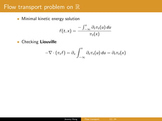
47. Flow transport problem on R
• Minimal kinetic energy solution
f (t, x) =
−
x
−∞
∂tπt(u) du
πt(x)
• Checking Liouville
− · (πtf ) = ∂x
x
−∞
∂tπt(u) du = ∂tπt(x)
A1 For f to be locally Lipschitz, assume
π0, L ∈ C1
(R, R+) =⇒ f ∈ C1
([0, 1] × R, R)
Jeremy Heng Flow transport 12/ 24

48. Flow transport problem on R
• Minimal kinetic energy solution
f (t, x) =
−
x
−∞
∂tπt(u) du
πt(x)
• Checking Liouville
− · (πtf ) = ∂x
x
−∞
∂tπt(u) du = ∂tπt(x)
A1 For f to be locally Lipschitz, assume
π0, L ∈ C1
(R, R+) =⇒ f ∈ C1
([0, 1] × R, R)
A2 For integrability of
1
0 Rd |f (t, x)|πt(x) dx dt < ∞, necessarily
|πtf |(t, x) =
x
−∞
∂tπt(u) du → 0 as |x| → ∞
since
∞
−∞
∂tπt(u) du = 0
Jeremy Heng Flow transport 12/ 24

49. Flow transport problem on R
• Minimal kinetic energy solution
f (t, x) =
−
x
−∞
∂tπt(u) du
πt(x)
• Checking Liouville
− · (πtf ) = ∂x
x
−∞
∂tπt(u) du = ∂tπt(x)
A1 For f to be locally Lipschitz, assume
π0, L ∈ C1
(R, R+) =⇒ f ∈ C1
([0, 1] × R, R)
A2 For integrability of
1
0 Rd |f (t, x)|πt(x) dx dt < ∞, necessarily
|πtf |(t, x) =
x
−∞
∂tπt(u) du → 0 as |x| → ∞
since
∞
−∞
∂tπt(u) du = 0
• Optimality: f = ϕ holds trivially
Jeremy Heng Flow transport 12/ 24

50. Flow transport problem on R
• Re-write solution as
f (t, x) =
λ (t)It {Ft(x) − Ix
t /It}
πt(x)
where Ix
t = Eπt
[1(−∞,x] log L(Xt)] and Ft is CDF of πt
Jeremy Heng Flow transport 13/ 24

51. Flow transport problem on R
• Re-write solution as
f (t, x) =
λ (t)It {Ft(x) − Ix
t /It}
πt(x)
where Ix
t = Eπt
[1(−∞,x] log L(Xt)] and Ft is CDF of πt
• Speed is controlled by λ (t) and πt(x)
Jeremy Heng Flow transport 13/ 24

52. Flow transport problem on R
• Re-write solution as
f (t, x) =
λ (t)It {Ft(x) − Ix
t /It}
πt(x)
where Ix
t = Eπt
[1(−∞,x] log L(Xt)] and Ft is CDF of πt
• Speed is controlled by λ (t) and πt(x)
• Sign is given by difference between Ft(x) and Ix
t /It ∈ [0, 1]
Jeremy Heng Flow transport 13/ 24

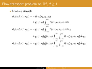
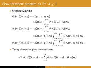
53. Flow transport problem on Rd
, d ≥ 1
• Multivariate solution for d = 3
(πtf1)(t, x1:3) = −
x1
−∞
∂tπt(u1, x2, x3) du1
+ g1(t, x1)
∞
−∞
∂tπt(u1, x2, x3) du1
(πtf2)(t, x1:3) = − g1(t, x1)
∞
−∞
x2
−∞
∂tπt(u1, u2, x3) du1:2
+ g1(t, x1)g2(t, x2)
∞
−∞
∞
−∞
∂tπt(u1, u2, x3) du1:2
(πtf3)(t, x1:3) = − g1(t, x1)g2(t, x2)
∞
−∞
∞
−∞
x3
−∞
∂tπt(u1, u2, u3) du1:3
where g1, g2 ∈ C2
([0, 1] × R, [0, 1])
Jeremy Heng Flow transport 14/ 24

54. Flow transport problem on Rd
, d ≥ 1
• Checking Liouville
∂x1 (πtf1)(t, x1:3) = − ∂tπt(x1, x2, x3)
+ g1(t, x1)
∞
−∞
∂tπt(u1, x2, x3) du1
∂x2
(πtf2)(t, x1:3) = − g1(t, x1)
∞
−∞
∂tπt(u1, x2, x3) du1:2
+ g1(t, x1)g2(t, x2)
∞
−∞
∞
−∞
∂tπt(u1, u2, x3) du1:2
∂x3
(πtf3)(t, x1:3) = − g1(t, x1)g2(t, x2)
∞
−∞
∞
−∞
∂tπt(u1, u2, x3) du1:2
Jeremy Heng Flow transport 15/ 24

55. Flow transport problem on Rd
, d ≥ 1
• Checking Liouville
∂x1 (πtf1)(t, x1:3) = − ∂tπt(x1, x2, x3)
+ g1(t, x1)
∞
−∞
∂tπt(u1, x2, x3) du1
∂x2
(πtf2)(t, x1:3) = − g1(t, x1)
∞
−∞
∂tπt(u1, x2, x3) du1:2
+ g1(t, x1)g2(t, x2)
∞
−∞
∞
−∞
∂tπt(u1, u2, x3) du1:2
∂x3
(πtf3)(t, x1:3) = − g1(t, x1)g2(t, x2)
∞
−∞
∞
−∞
∂tπt(u1, u2, x3) du1:2
• Taking divergence gives telescopic sum
− · (πtf )(t, x1:3) = −
3
i=1
∂xi
(πtfi )(t, x1:3) = ∂tπt(x1:3)
Jeremy Heng Flow transport 15/ 24

56. Flow transport problem on Rd
, d ≥ 1
A1 For f to be locally Lipschitz, assume
π0, L ∈ C1
(Rd
, R+) =⇒ f ∈ C1
([0, 1] × Rd
, Rd
)
Jeremy Heng Flow transport 16/ 24

57. Flow transport problem on Rd
, d ≥ 1
A1 For f to be locally Lipschitz, assume
π0, L ∈ C1
(Rd
, R+) =⇒ f ∈ C1
([0, 1] × Rd
, Rd
)
A2 For integrability of
1
0 Rd |f (t, x)|πt(x) dx dt < ∞, necessarily
|πtf |(t, x)| → 0 as |x| → ∞
if {gi } are non-decreasing functions with tail behaviour
gi (t, xi ) → 0 as xi → −∞,
gi (t, xi ) → 1 as xi → ∞
Jeremy Heng Flow transport 16/ 24

58. Flow transport problem on Rd
, d ≥ 1
A1 For f to be locally Lipschitz, assume
π0, L ∈ C1
(Rd
, R+) =⇒ f ∈ C1
([0, 1] × Rd
, Rd
)
A2 For integrability of
1
0 Rd |f (t, x)|πt(x) dx dt < ∞, necessarily
|πtf |(t, x)| → 0 as |x| → ∞
if {gi } are non-decreasing functions with tail behaviour
gi (t, xi ) → 0 as xi → −∞,
gi (t, xi ) → 1 as xi → ∞
• Choosing gi (t, xi ) = Ft(xi ) as marginal CDF of πt allows f to
decouple if distributions are independent
Jeremy Heng Flow transport 16/ 24

59. Approximate Gibbs flow transport
• Solution involved integrals of increasing dimension as it tracks
increasing conditional distributions
πt(x1|x2:d ), πt(x2|3:d ), . . . , πt(xd ), xi ∈ R
Jeremy Heng Flow transport 17/ 24

60. Approximate Gibbs flow transport
• Solution involved integrals of increasing dimension as it tracks
increasing conditional distributions
πt(x1|x2:d ), πt(x2|3:d ), . . . , πt(xd ), xi ∈ R
• Trade-off accuracy for computational tractability: track full
conditional distributions
πt(xi |x−i ), xi ∈ Rdi
Jeremy Heng Flow transport 17/ 24

61. Approximate Gibbs flow transport
• Solution involved integrals of increasing dimension as it tracks
increasing conditional distributions
πt(x1|x2:d ), πt(x2|3:d ), . . . , πt(xd ), xi ∈ R
• Trade-off accuracy for computational tractability: track full
conditional distributions
πt(xi |x−i ), xi ∈ Rdi
• System of Liouville equations
− xi
· πt(xi |x−i )˜fi (t, x) = ∂tπt(xi |x−i ),
each defined on (0, 1) × Rdi
Jeremy Heng Flow transport 17/ 24

62. Approximate Gibbs flow transport
• For di = 1, solution is
˜fi (t, x) =
−
xi
−∞
∂tπt(ui |x−i ) dui
πt(xi |x−i )
Jeremy Heng Flow transport 18/ 24

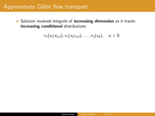
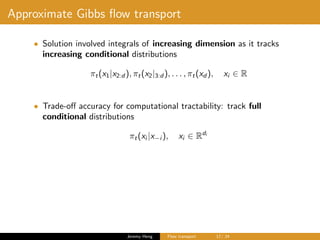
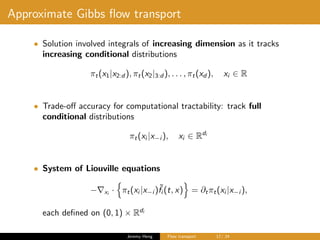
63. Approximate Gibbs flow transport
• For di = 1, solution is
˜fi (t, x) =
−
xi
−∞
∂tπt(ui |x−i ) dui
πt(xi |x−i )
• If π0, L ∈ C1
(Rd
, R+) and lim|x|→∞ L(x) = 0, the ODE
dXt = ˜f (t, Xt)dt, X0 ∼ π0
admits a unique solution on [0, 1], referred to as Gibbs flow
Jeremy Heng Flow transport 18/ 24

64. Approximate Gibbs flow transport
• For di = 1, solution is
˜fi (t, x) =
−
xi
−∞
∂tπt(ui |x−i ) dui
πt(xi |x−i )
• If π0, L ∈ C1
(Rd
, R+) and lim|x|→∞ L(x) = 0, the ODE
dXt = ˜f (t, Xt)dt, X0 ∼ π0
admits a unique solution on [0, 1], referred to as Gibbs flow
• For di > 1, can often exploit analytical tractability of πt(xi |x−i ) to
solve for ˜fi (t, x); or apply multivariate extension
Jeremy Heng Flow transport 18/ 24

65. Approximate Gibbs flow transport
• For di = 1, solution is
˜fi (t, x) =
−
xi
−∞
∂tπt(ui |x−i ) dui
πt(xi |x−i )
• If π0, L ∈ C1
(Rd
, R+) and lim|x|→∞ L(x) = 0, the ODE
dXt = ˜f (t, Xt)dt, X0 ∼ π0
admits a unique solution on [0, 1], referred to as Gibbs flow
• For di > 1, can often exploit analytical tractability of πt(xi |x−i ) to
solve for ˜fi (t, x); or apply multivariate extension
• Otherwise, analogous to Metropolis-within-Gibbs, split into one
dimensional components and apply above
Jeremy Heng Flow transport 18/ 24

66. Error control
• Define local error
εt(x) = ∂tπt(x) + · (πt(x)˜f (t, x))
= ∂tπt(x) −
p
i=1
∂tπt(xi |x−i )πt(x−i )
Jeremy Heng Flow transport 19/ 24

67. Error control
• Define local error
εt(x) = ∂tπt(x) + · (πt(x)˜f (t, x))
= ∂tπt(x) −
p
i=1
∂tπt(xi |x−i )πt(x−i )
• Gibbs flow exploits local independence:
πt(x) =
p
i=1
πt(xi ) =⇒ εt(x) = 0
Jeremy Heng Flow transport 19/ 24

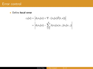
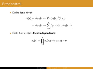
68. Error control
• Define local error
εt(x) = ∂tπt(x) + · (πt(x)˜f (t, x))
= ∂tπt(x) −
p
i=1
∂tπt(xi |x−i )πt(x−i )
• Gibbs flow exploits local independence:
πt(x) =
p
i=1
πt(xi ) =⇒ εt(x) = 0
• If Gibbs flow induces {˜πt}t∈[0,1] with ˜π0 = π0
˜πt − πt
2
L2 ≤ t
t
0
εu
2
L2 du · exp 1 +
t
0
· ˜f (u, ·) ∞ du
Jeremy Heng Flow transport 19/ 24

69. Numerical integration of Gibbs flow
• Previously, we considered the forward Euler scheme
Ym = Ym−1 + ∆t ˜f (tm−1, Ym−1) = Φm(Ym−1)
Jeremy Heng Flow transport 20/ 24

70. Numerical integration of Gibbs flow
• Previously, we considered the forward Euler scheme
Ym = Ym−1 + ∆t ˜f (tm−1, Ym−1) = Φm(Ym−1)
• To get Law(Ym), we need Jacobian determinant of Φm which
typically costs O(d3
) for di = 1
Jeremy Heng Flow transport 20/ 24

71. Numerical integration of Gibbs flow
• Previously, we considered the forward Euler scheme
Ym = Ym−1 + ∆t ˜f (tm−1, Ym−1) = Φm(Ym−1)
• To get Law(Ym), we need Jacobian determinant of Φm which
typically costs O(d3
) for di = 1
• In contrast, this scheme mimicking a systematic Gibbs scan
Ym[i] = Ym−1[i] + ∆t ˜f (tm−1, Ym[1 : i − 1], Ym−1[i : p])
Ym = Φm,d ◦ · · · ◦ Φm,1(Ym−1)
is also order one, and costs O(d)
Jeremy Heng Flow transport 20/ 24

72. Mixture modelling example
• Lack of identifiability induces π on R4
with 4! = 24 well-separated
and identical modes
Jeremy Heng Flow transport 21/ 24

73. Mixture modelling example
• Lack of identifiability induces π on R4
with 4! = 24 well-separated
and identical modes
• Gibbs flow approximation
t =0.0006
x1
x2
−10 −5 0 5 10
−10
−5
0
5
10
t =0.0058
x1
x2
−10 −5 0 5 10
−10
−5
0
5
10
t =0.0542
x1
x2
−10 −5 0 5 10
−10
−5
0
5
10
t =1.0000
x1
x2
−10 −5 0 5 10
−10
−5
0
5
10
Jeremy Heng Flow transport 21/ 24

74. Mixture modelling example
• Proportion of particles in each of the 24 modes
0.00
0.01
0.02
0.03
0.04
1 2 3 4 5 6 7 8 9 101112131415161718192021222324
Mode
Proportionofparticles
Jeremy Heng Flow transport 22/ 24

75. Mixture modelling example
• Proportion of particles in each of the 24 modes
0.00
0.01
0.02
0.03
0.04
1 2 3 4 5 6 7 8 9 101112131415161718192021222324
Mode
Proportionofparticles
• Pearson’s Chi-squared test for uniformity gives p-value of 0.85
Jeremy Heng Flow transport 22/ 24

76. Cox point process model
• Effective sample size % in dimension d
0
25
50
75
100
0.00 0.25 0.50 0.75 1.00
time
ESS%
method AIS GF−SIS GF−AIS
d = 100
0
25
50
75
100
0.00 0.25 0.50 0.75 1.00
time
ESS%
method AIS GF−SIS GF−AIS
d = 225
0
25
50
75
100
0.00 0.25 0.50 0.75 1.00
time
ESS%
method AIS GF−SIS GF−AIS
d = 400
Jeremy Heng Flow transport 23/ 24

77. Cox point process model
• Effective sample size % in dimension d
• AIS: AIS with HMC moves
0
25
50
75
100
0.00 0.25 0.50 0.75 1.00
time
ESS%
method AIS GF−SIS GF−AIS
d = 100
0
25
50
75
100
0.00 0.25 0.50 0.75 1.00
time
ESS%
method AIS GF−SIS GF−AIS
d = 225
0
25
50
75
100
0.00 0.25 0.50 0.75 1.00
time
ESS%
method AIS GF−SIS GF−AIS
d = 400
Jeremy Heng Flow transport 23/ 24

78. Cox point process model
• Effective sample size % in dimension d
• AIS: AIS with HMC moves
• GF-SIS: Gibbs flow
0
25
50
75
100
0.00 0.25 0.50 0.75 1.00
time
ESS%
method AIS GF−SIS GF−AIS
d = 100
0
25
50
75
100
0.00 0.25 0.50 0.75 1.00
time
ESS%
method AIS GF−SIS GF−AIS
d = 225
0
25
50
75
100
0.00 0.25 0.50 0.75 1.00
time
ESS%
method AIS GF−SIS GF−AIS
d = 400
Jeremy Heng Flow transport 23/ 24

79. Cox point process model
• Effective sample size % in dimension d
• AIS: AIS with HMC moves
• GF-SIS: Gibbs flow
• GF-AIS: Gibbs flow with HMC moves
0
25
50
75
100
0.00 0.25 0.50 0.75 1.00
time
ESS%
method AIS GF−SIS GF−AIS
d = 100
0
25
50
75
100
0.00 0.25 0.50 0.75 1.00
time
ESS%
method AIS GF−SIS GF−AIS
d = 225
0
25
50
75
100
0.00 0.25 0.50 0.75 1.00
time
ESS%
method AIS GF−SIS GF−AIS
d = 400
Jeremy Heng Flow transport 23/ 24

80. End
• Heng, J., Doucet, A., & Pokern, Y. (2015). Gibbs Flow for
Approximate Transport with Applications to Bayesian Computation.
arXiv preprint arXiv:1509.08787.
• Updated article and R package coming soon!
Jeremy Heng Flow transport 24/ 24