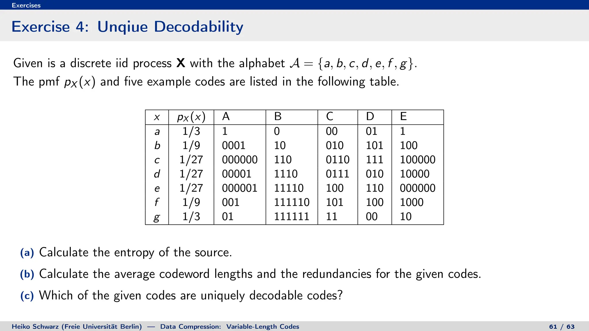
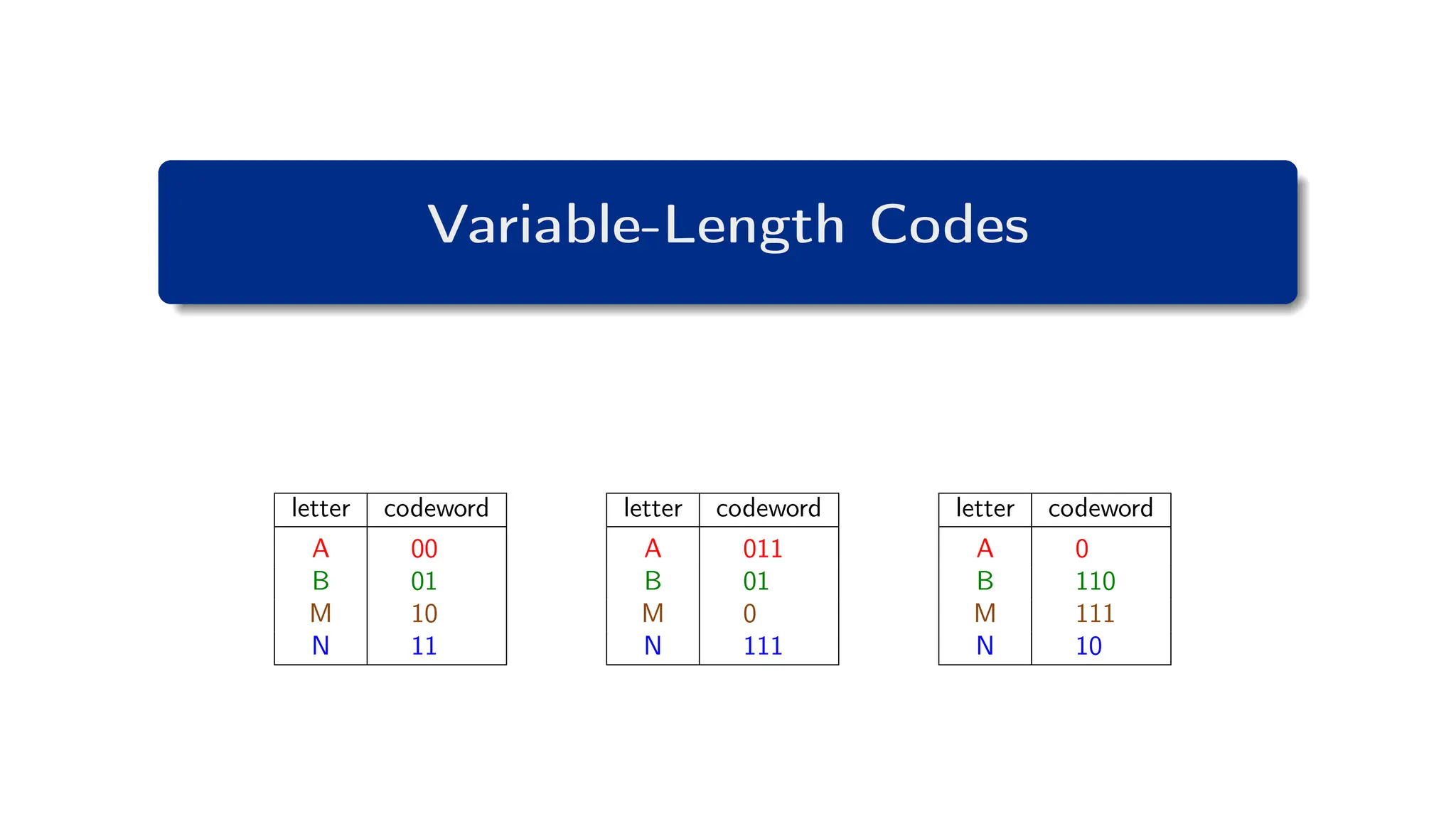
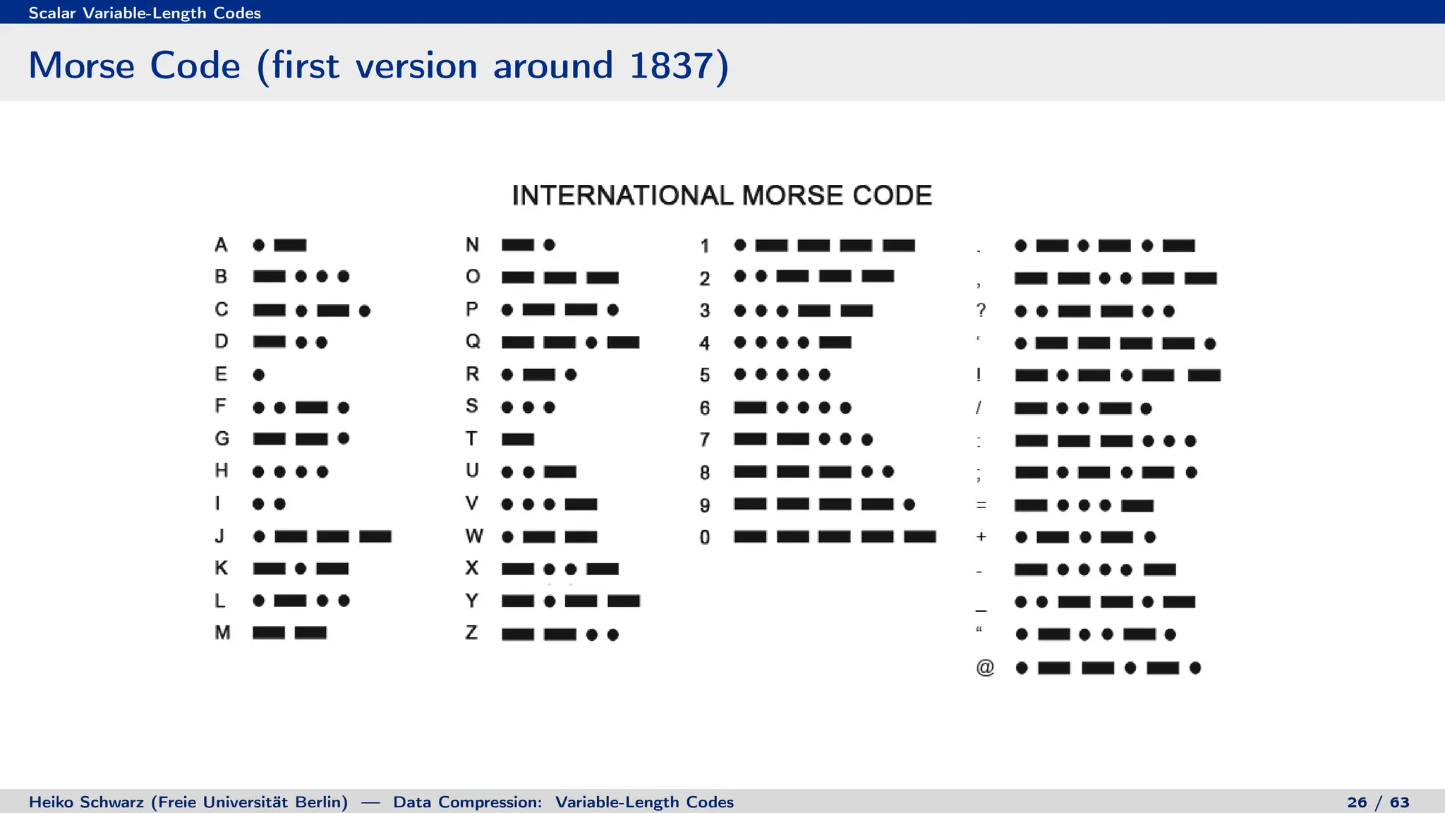
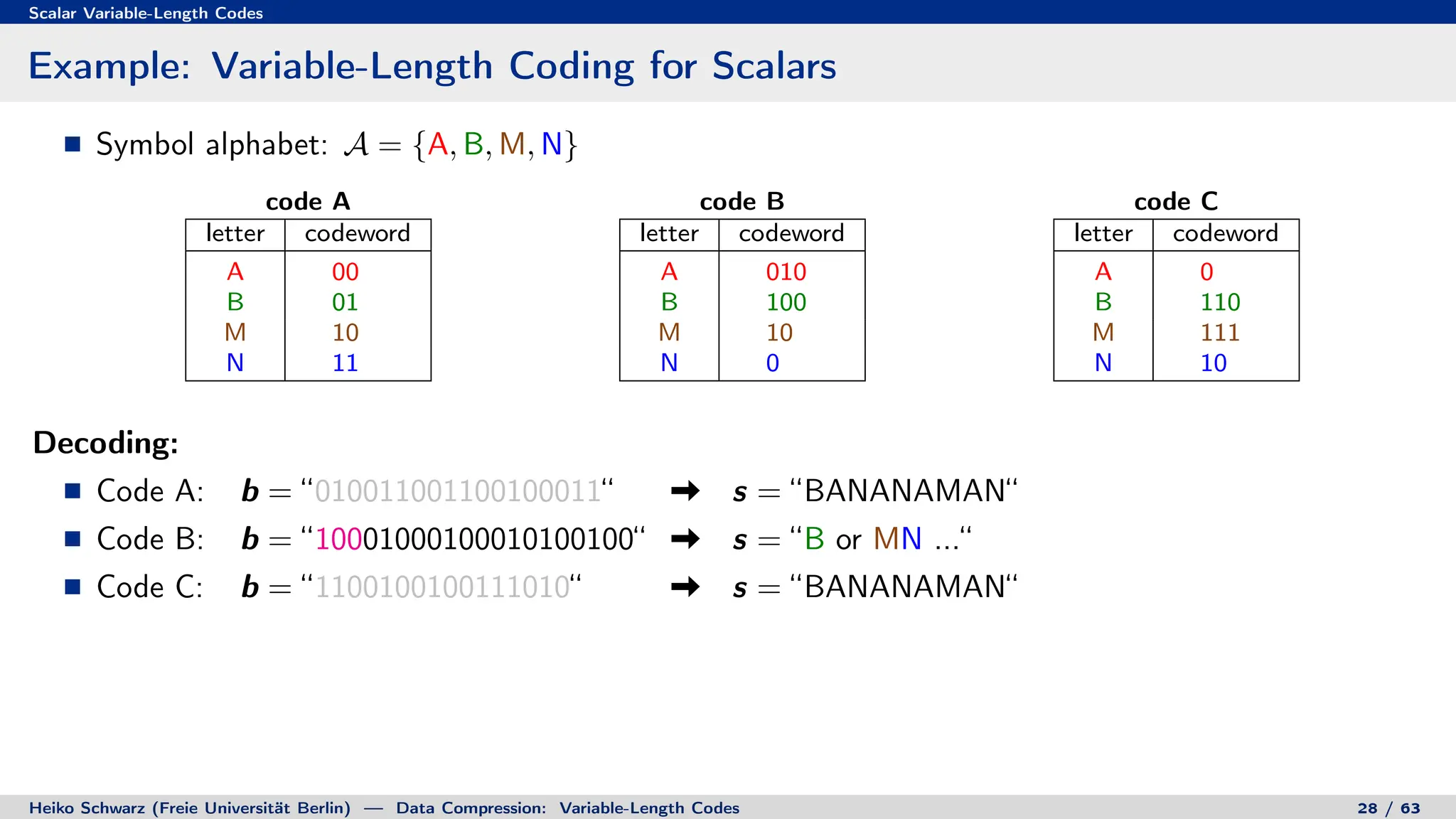
Variable-length codes can be used to encode letters or symbols using codewords of varying lengths. The document reviews mathematical basics relevant to analyzing source coding and data compression, including:
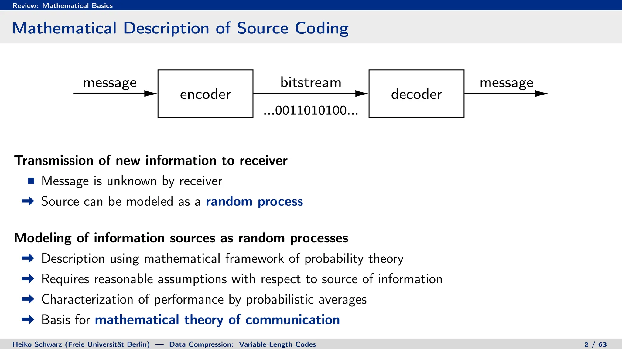
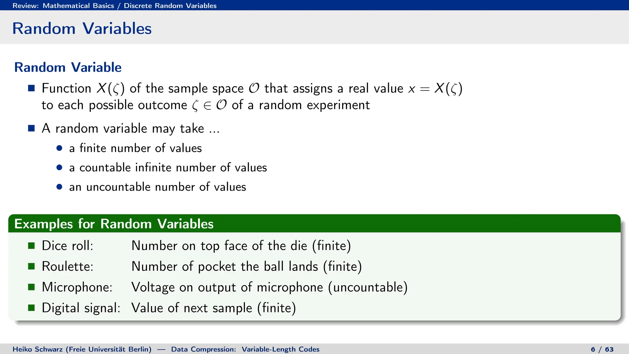
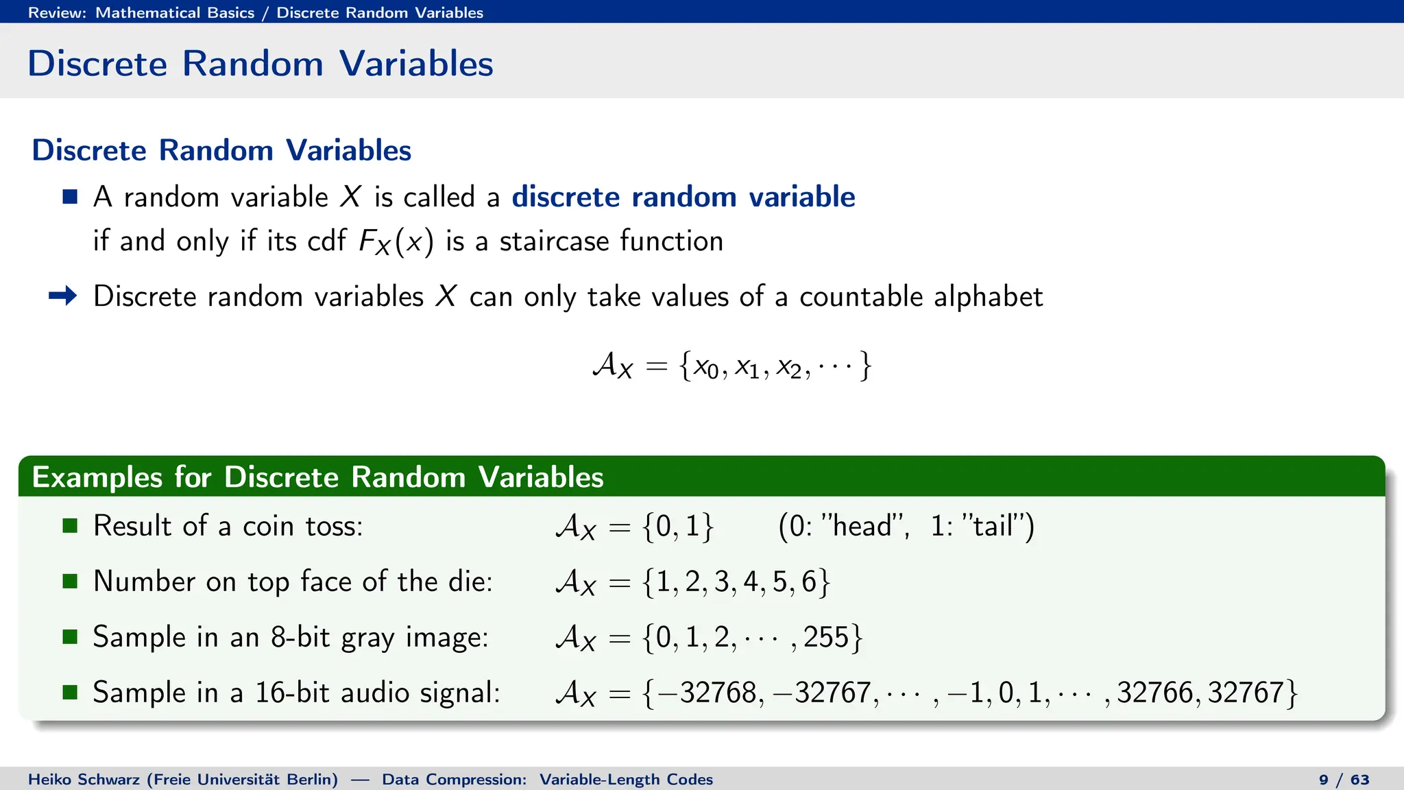
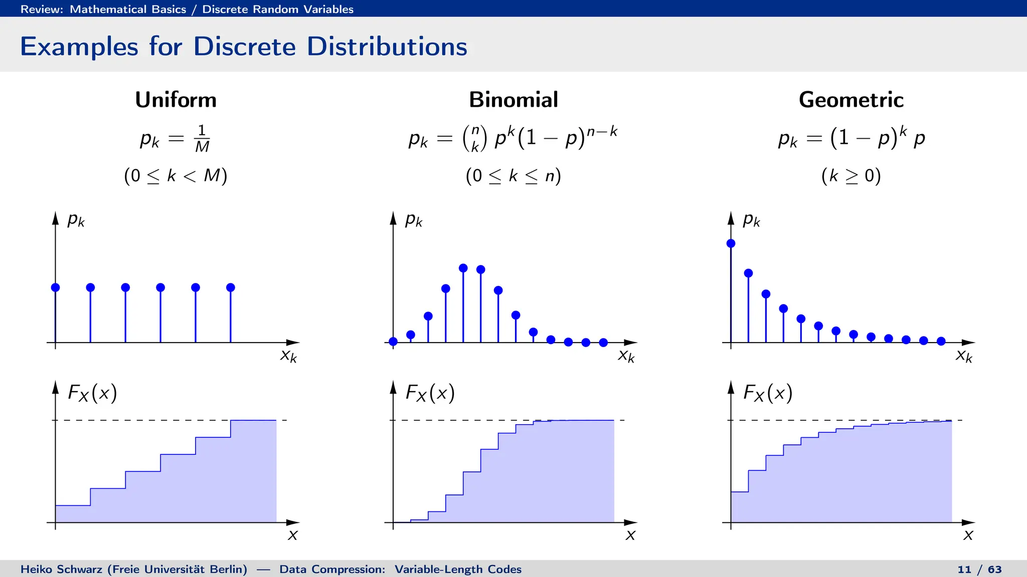
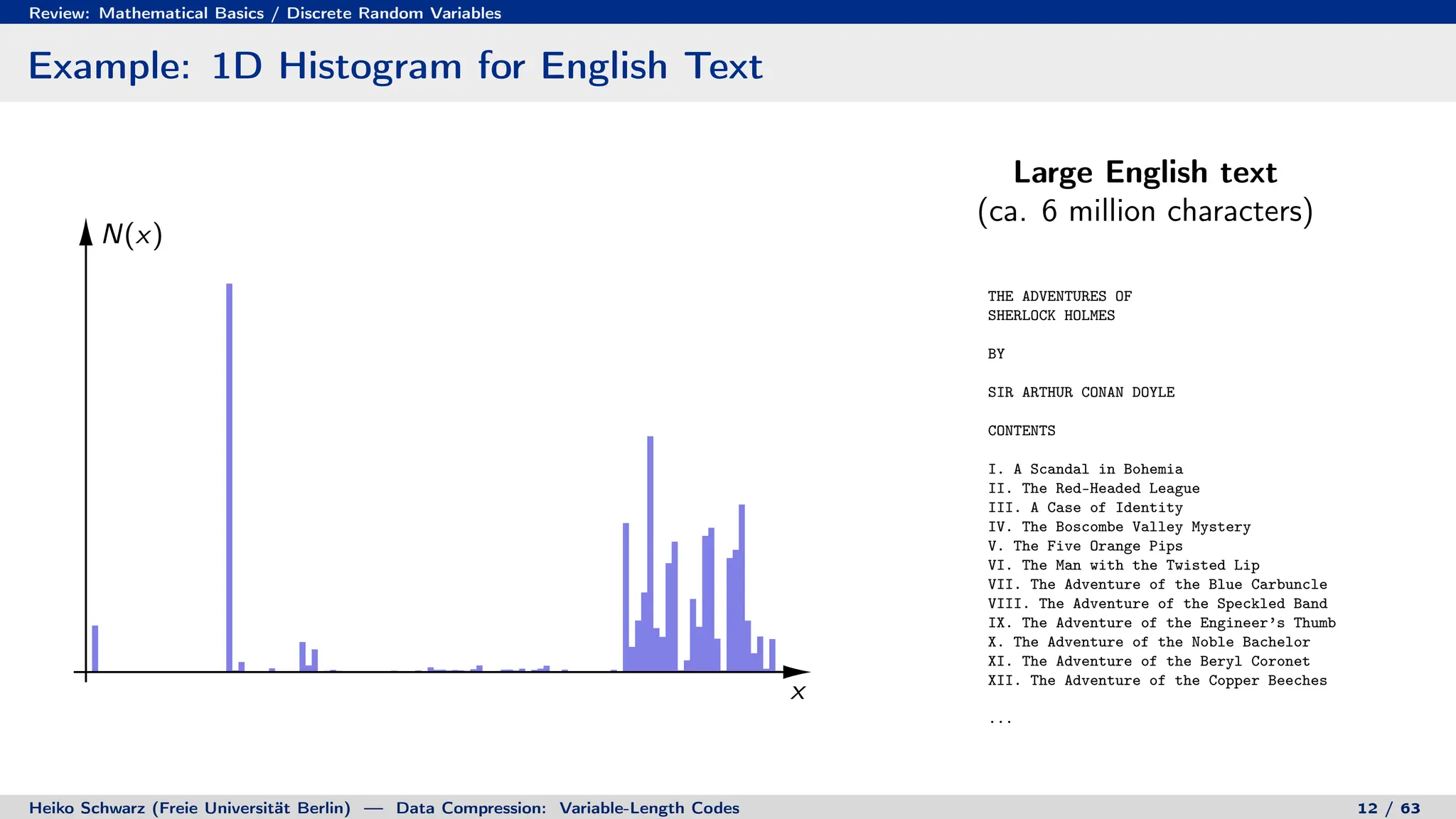
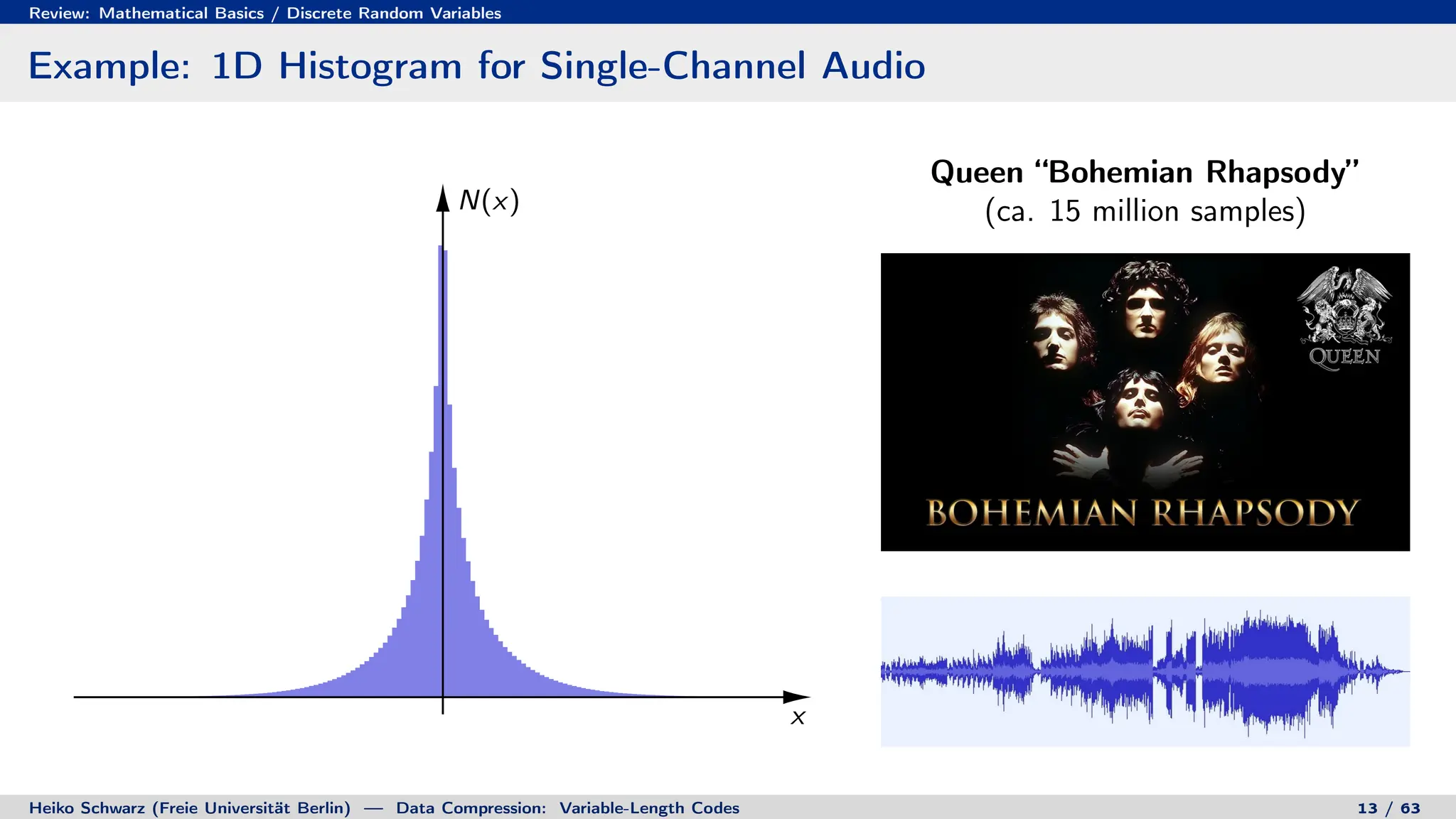
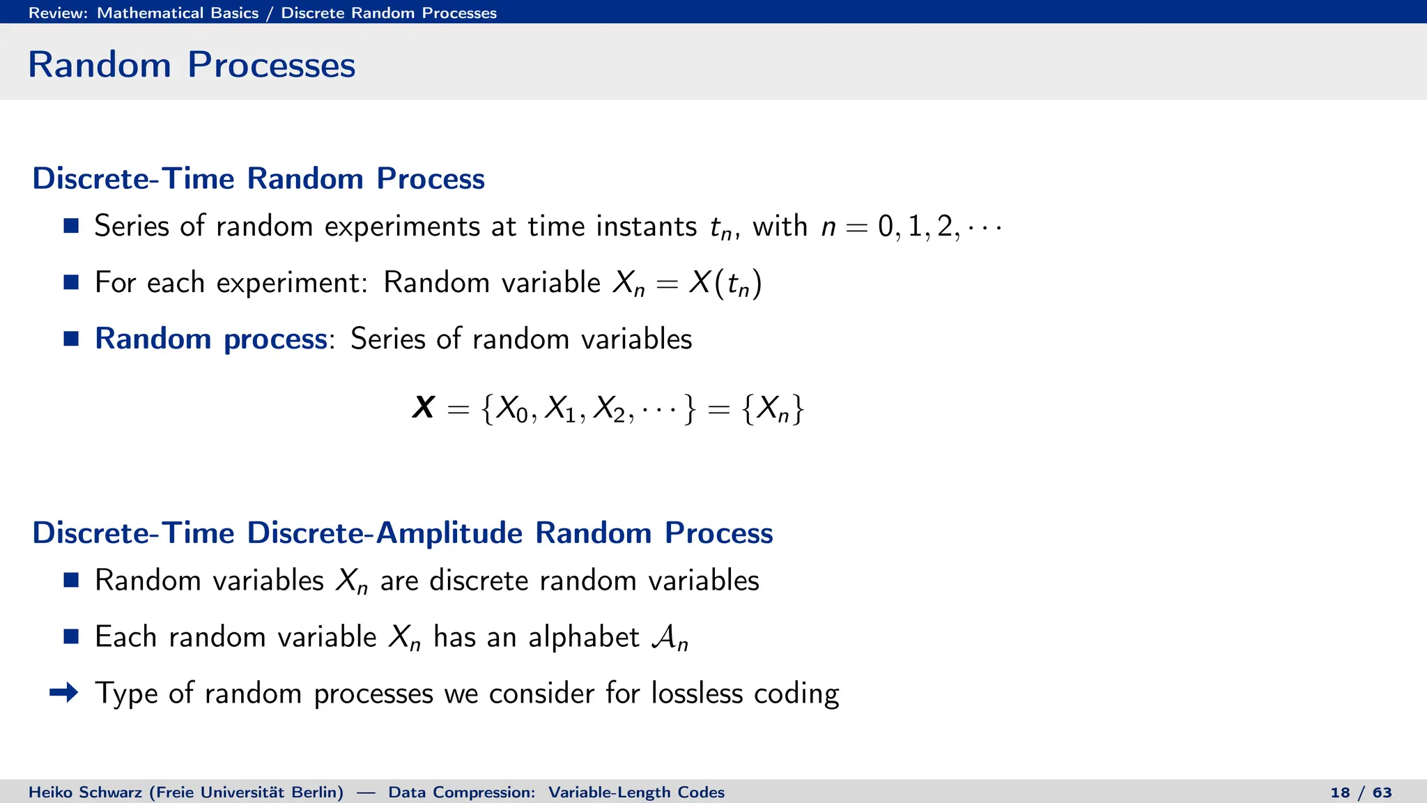
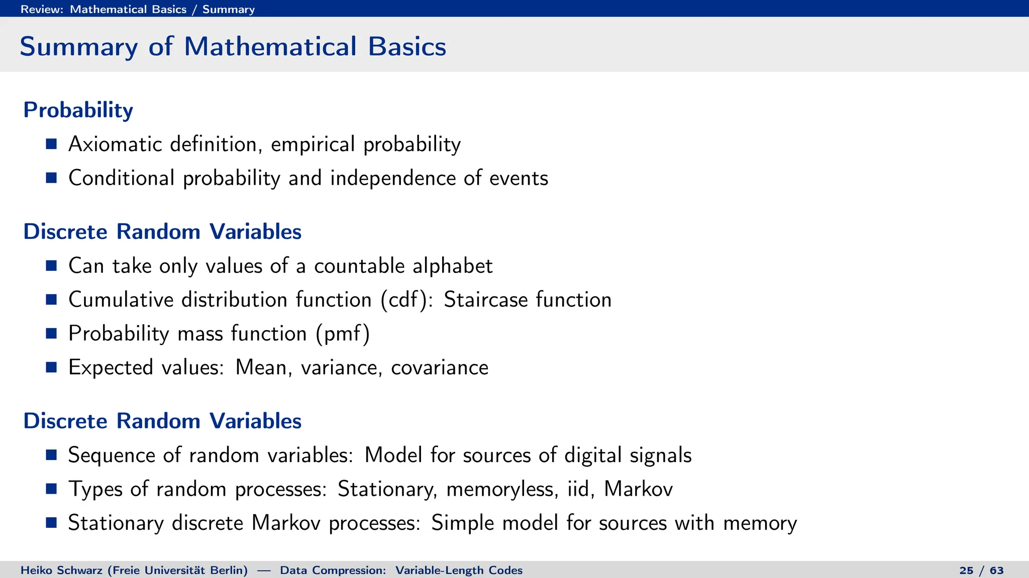
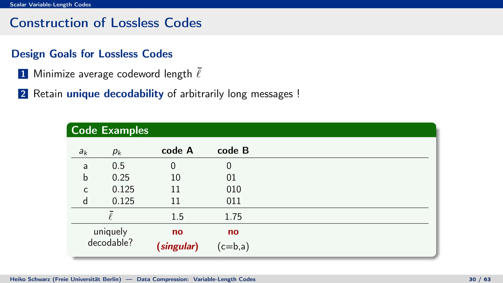
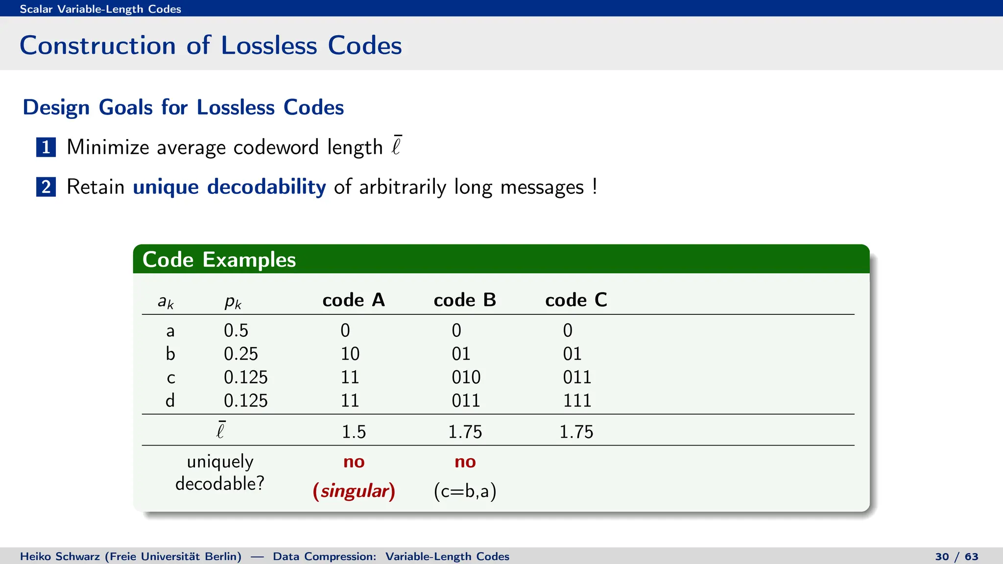
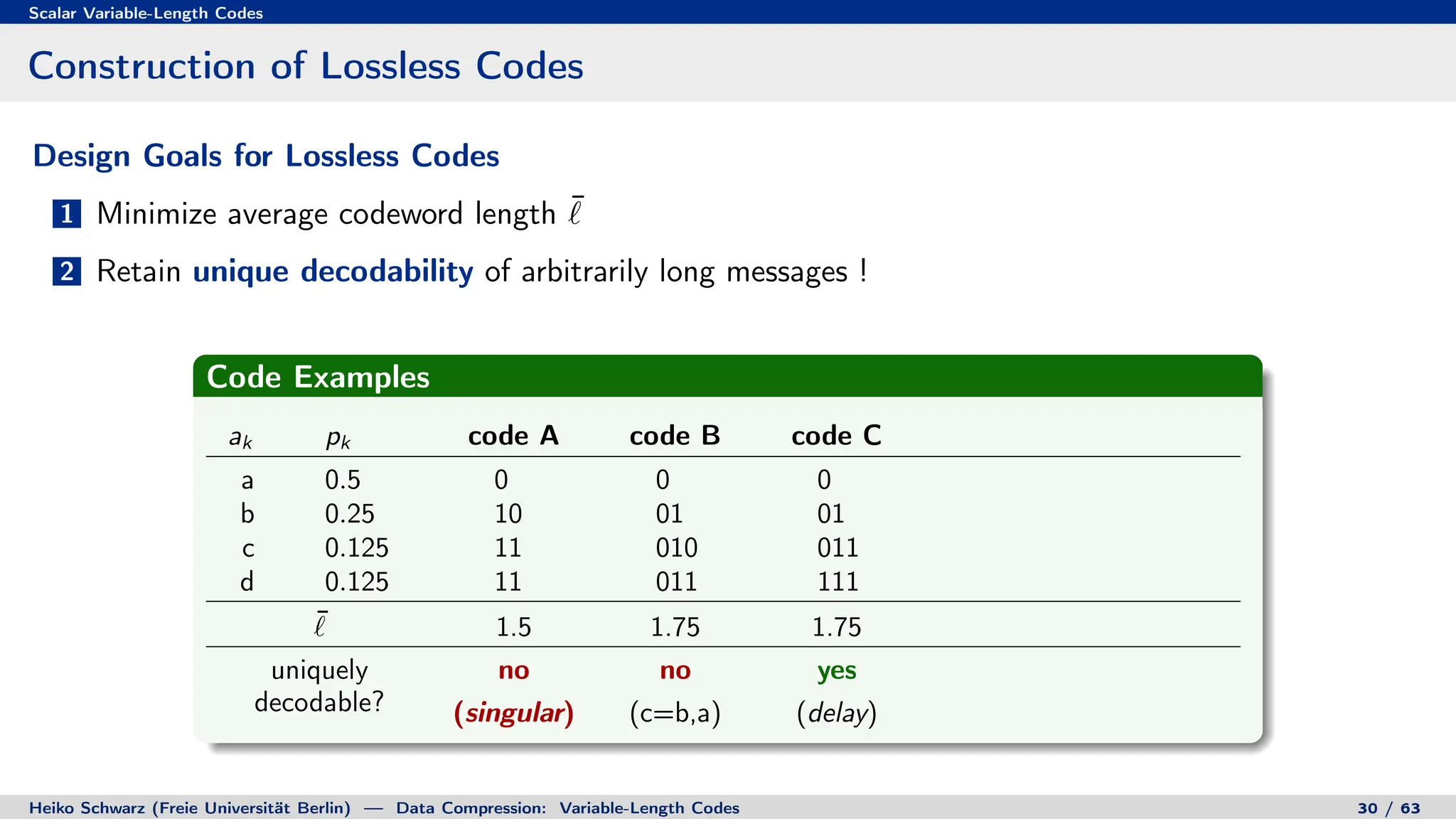
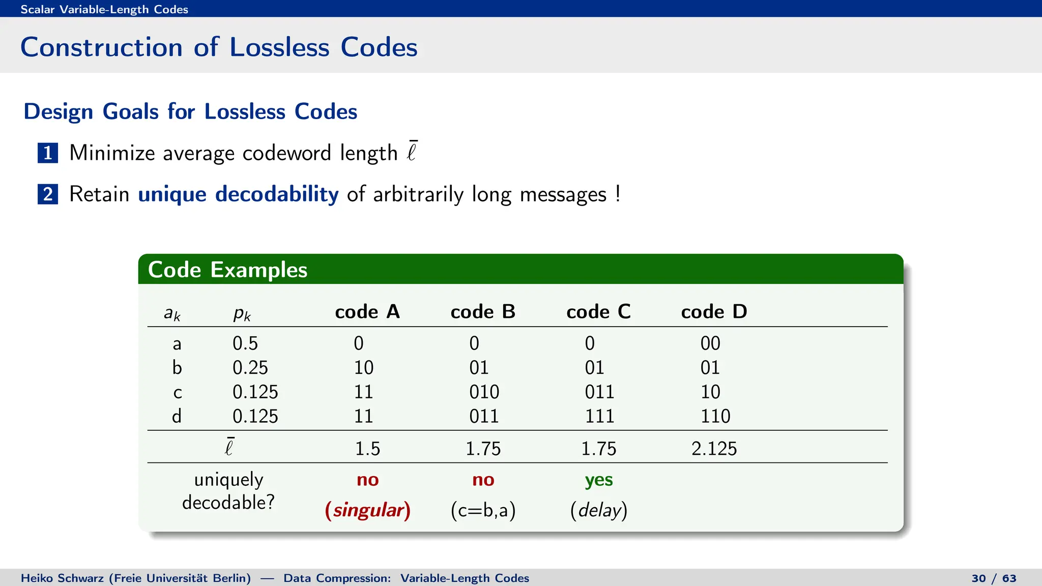
1. Discrete random variables and processes can be used to model information sources as sequences of random outcomes.
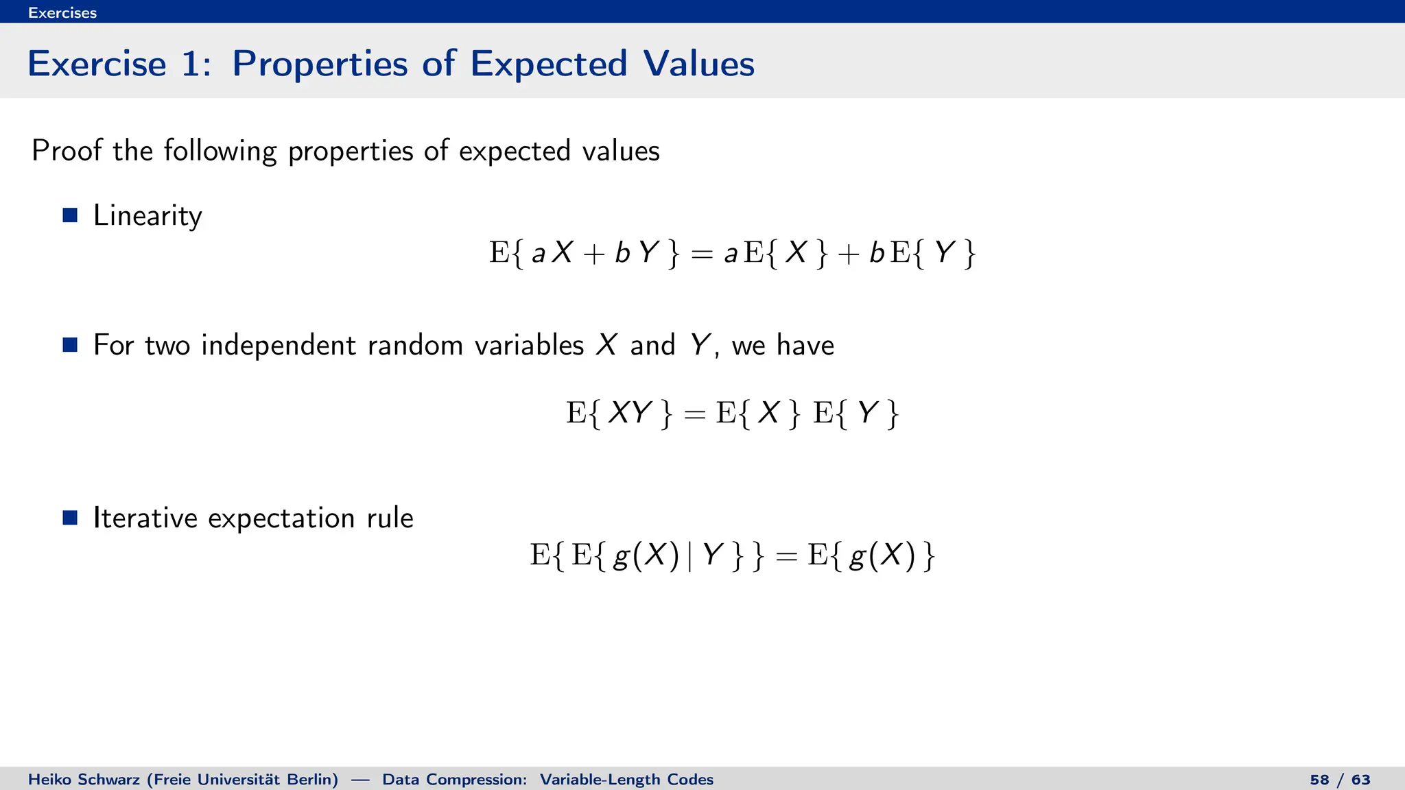
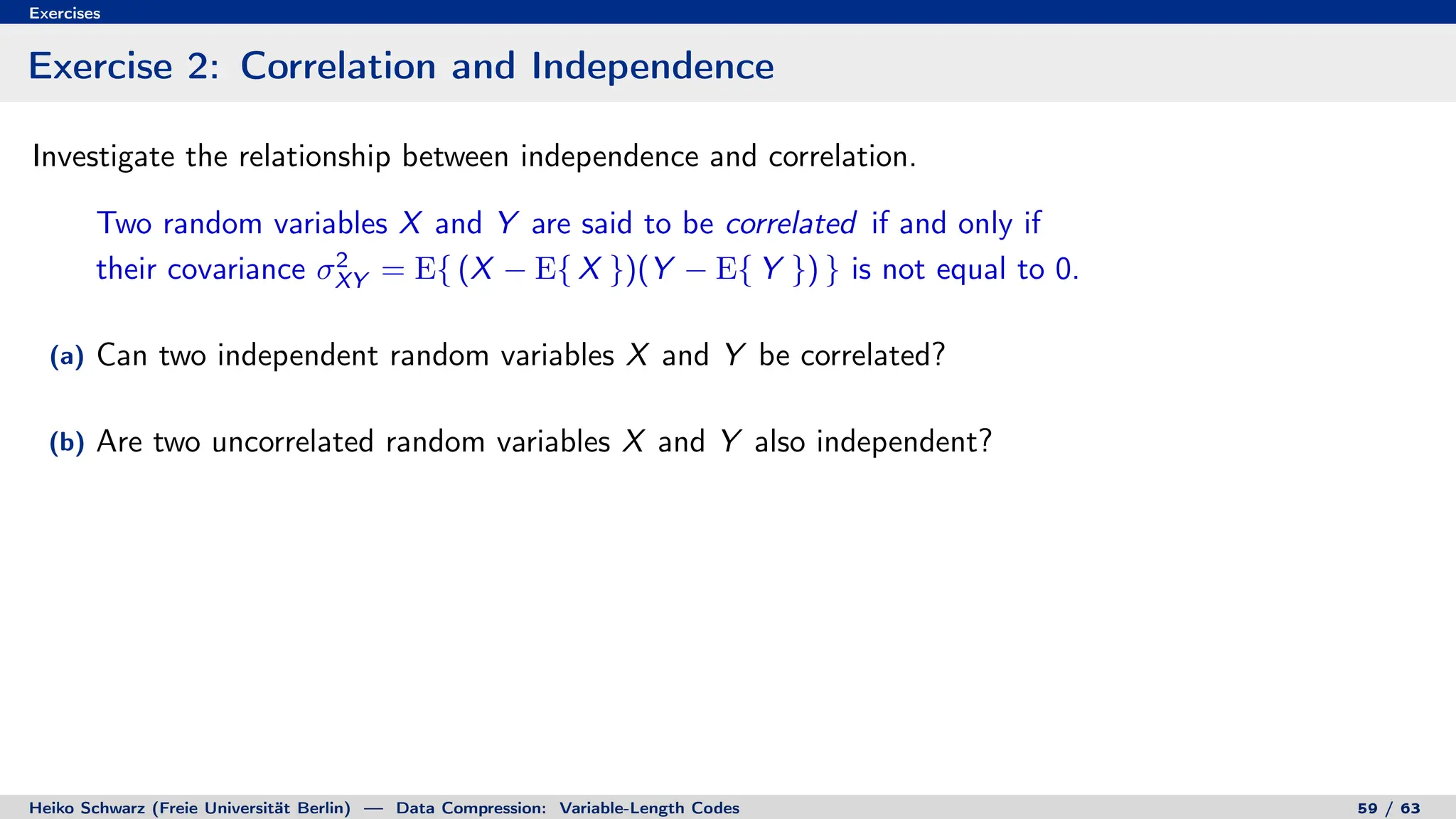
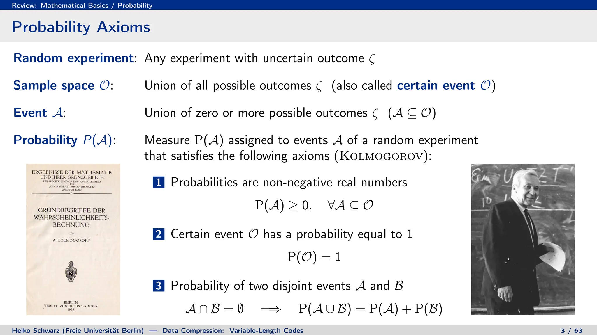
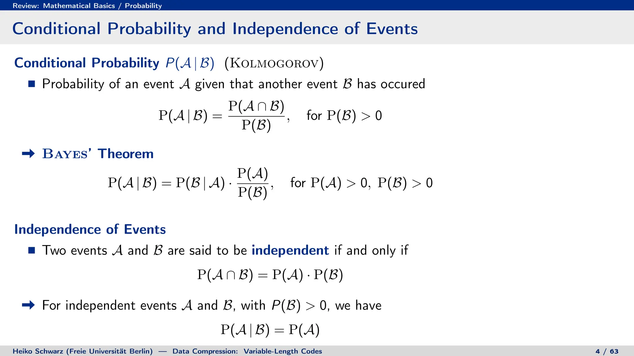
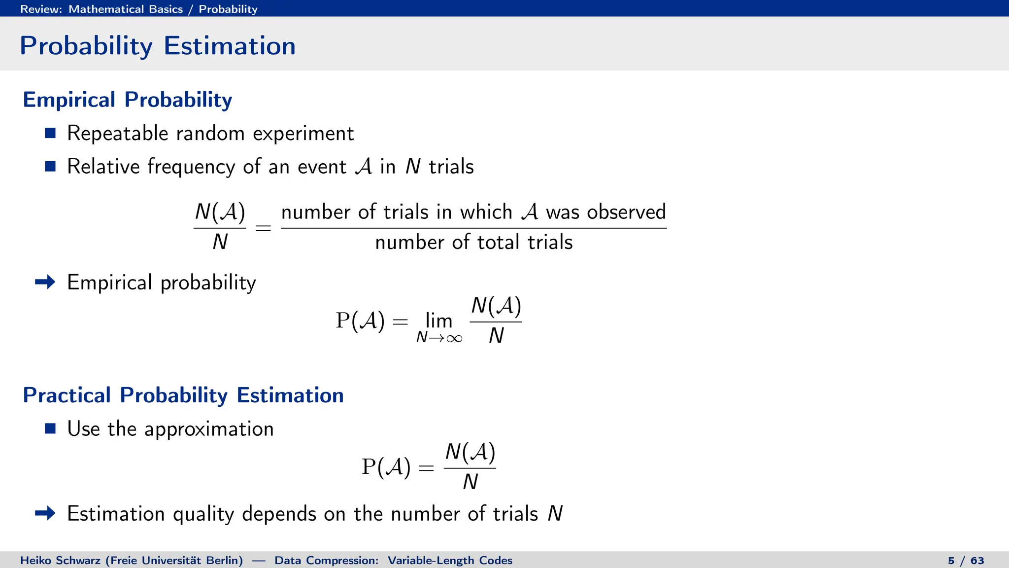
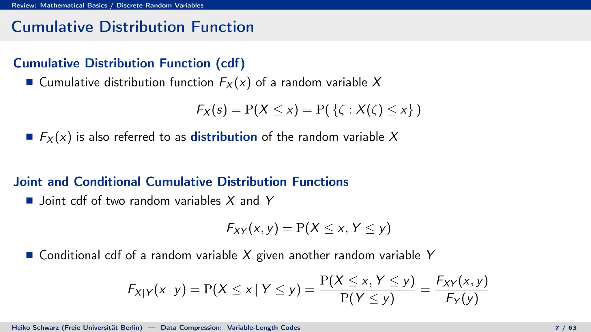
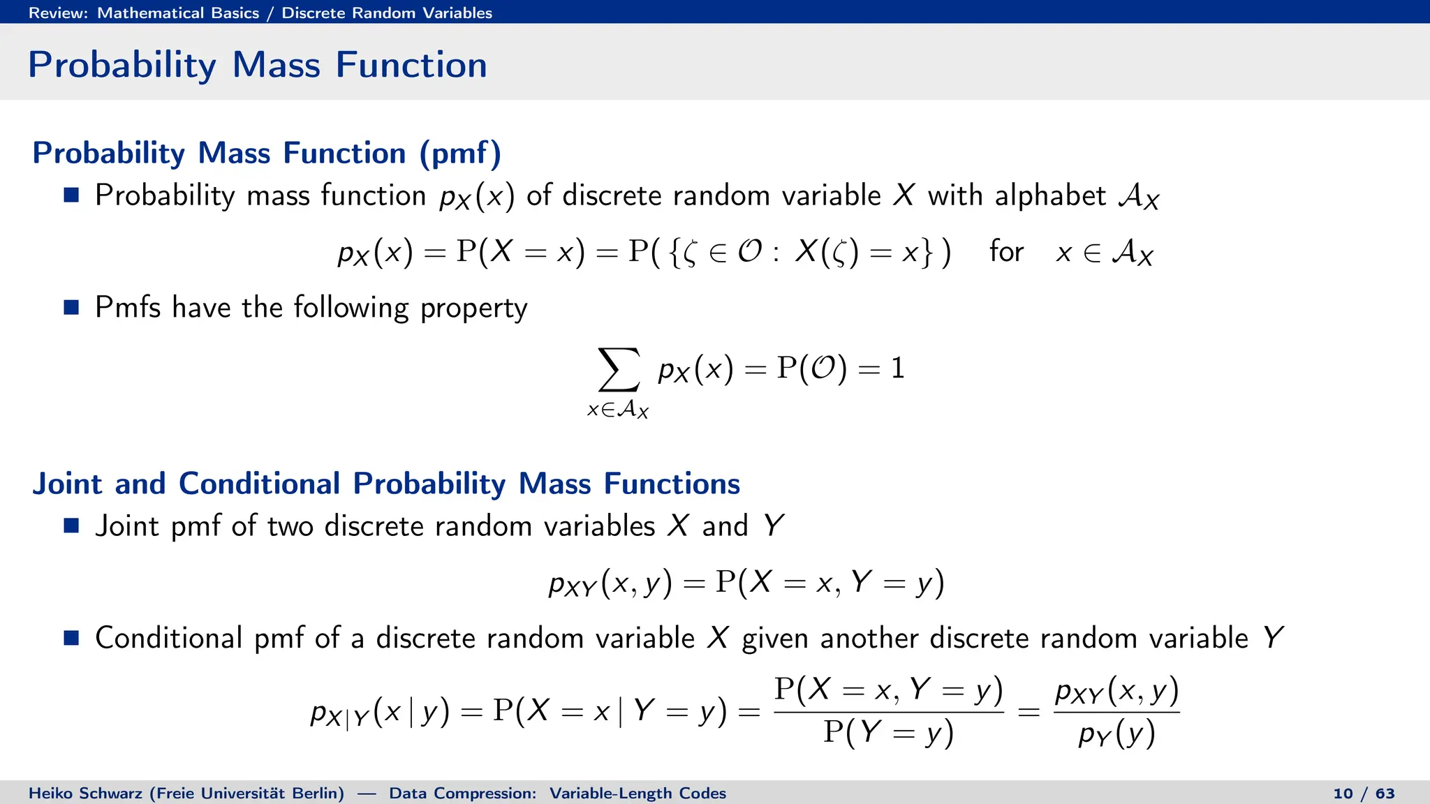
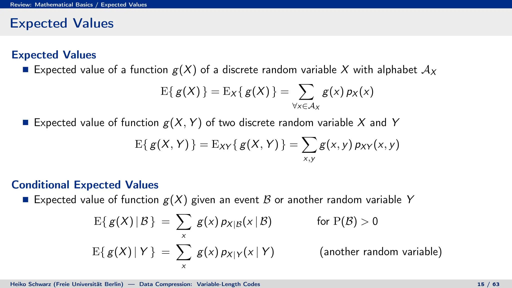
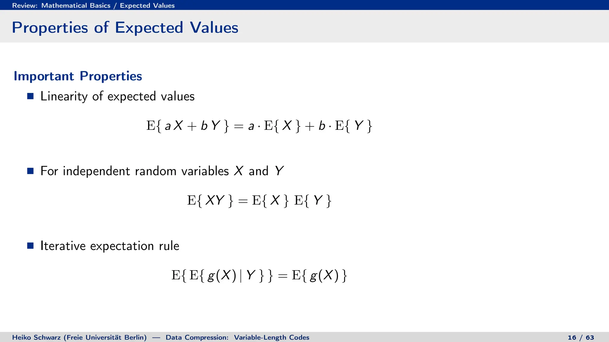
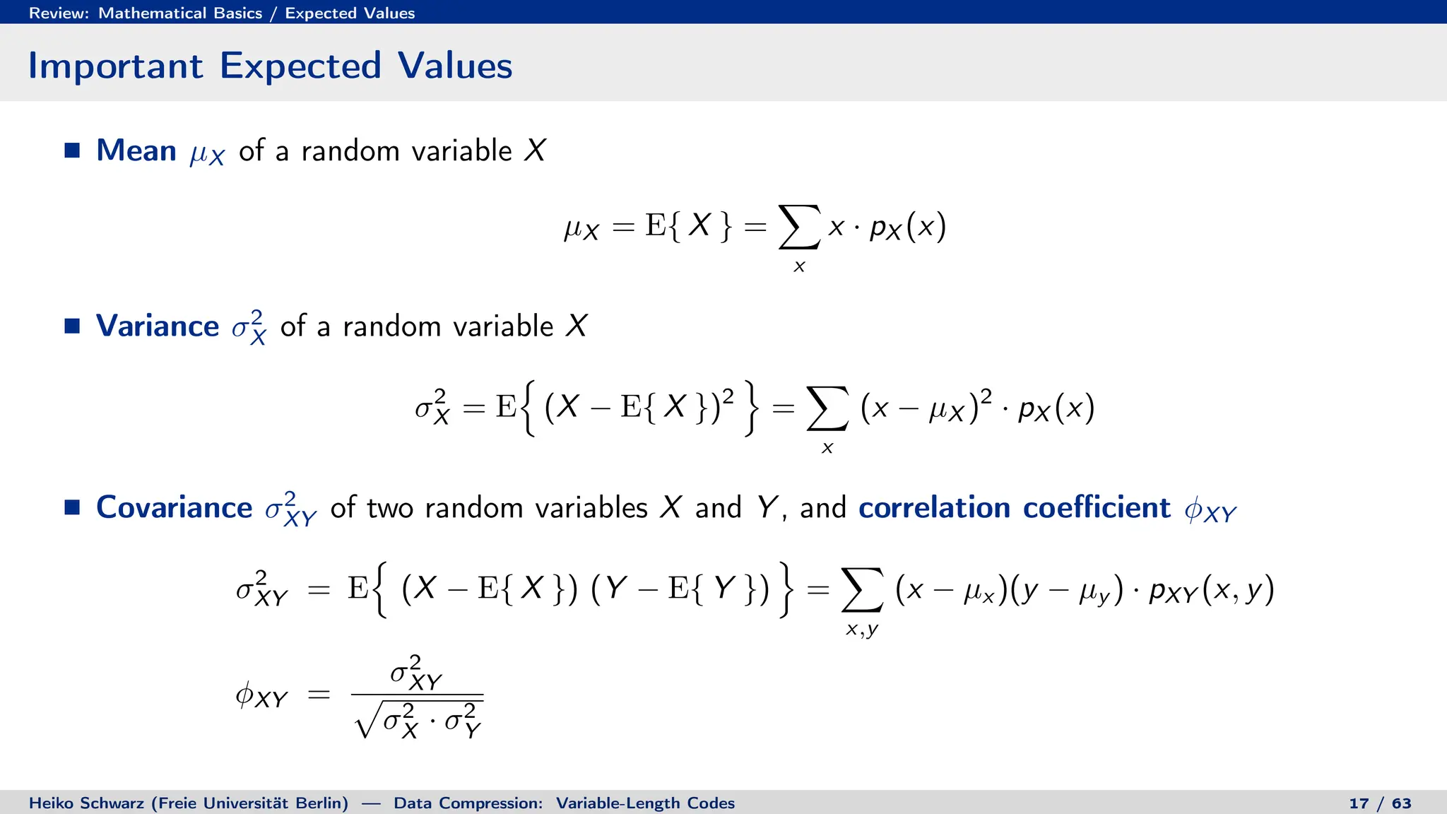
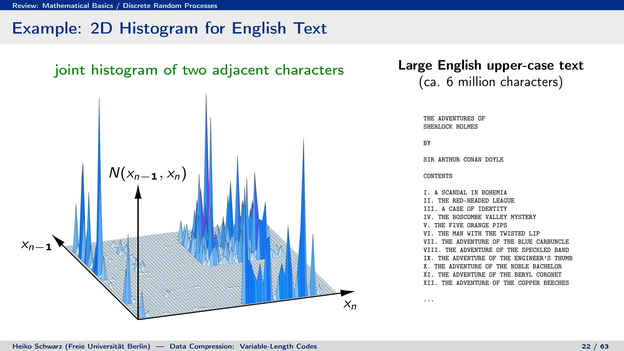
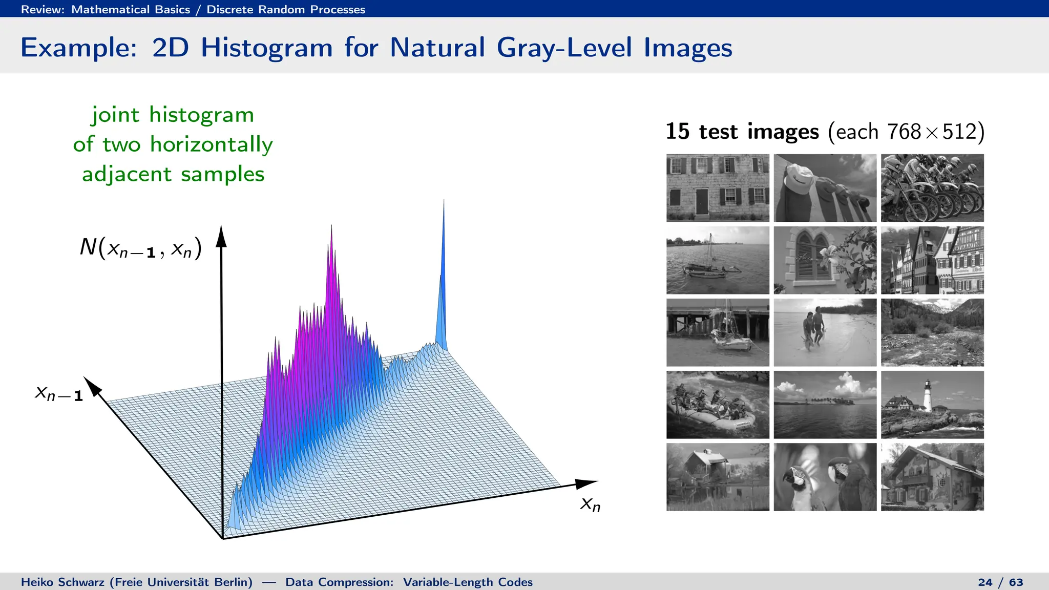
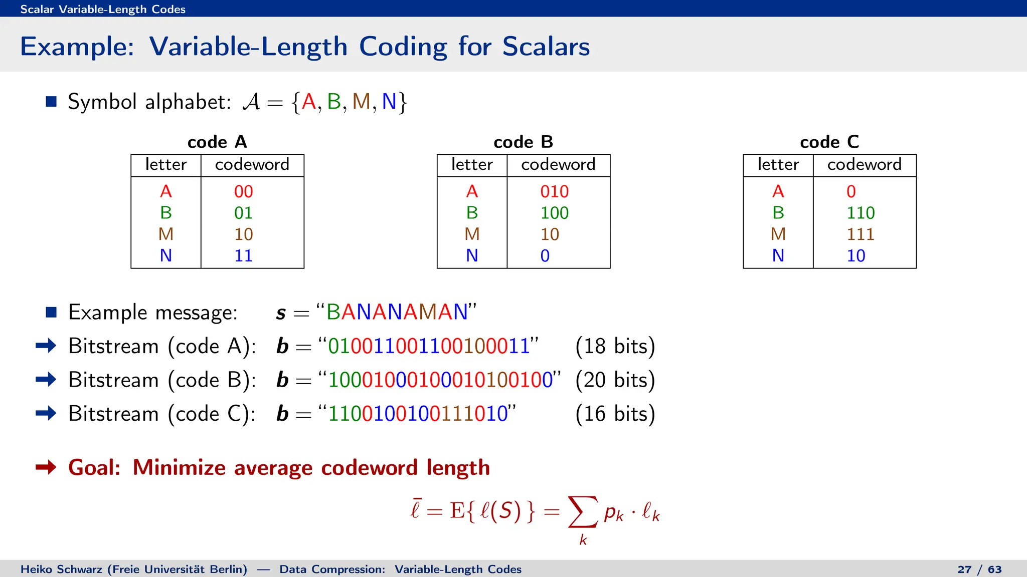
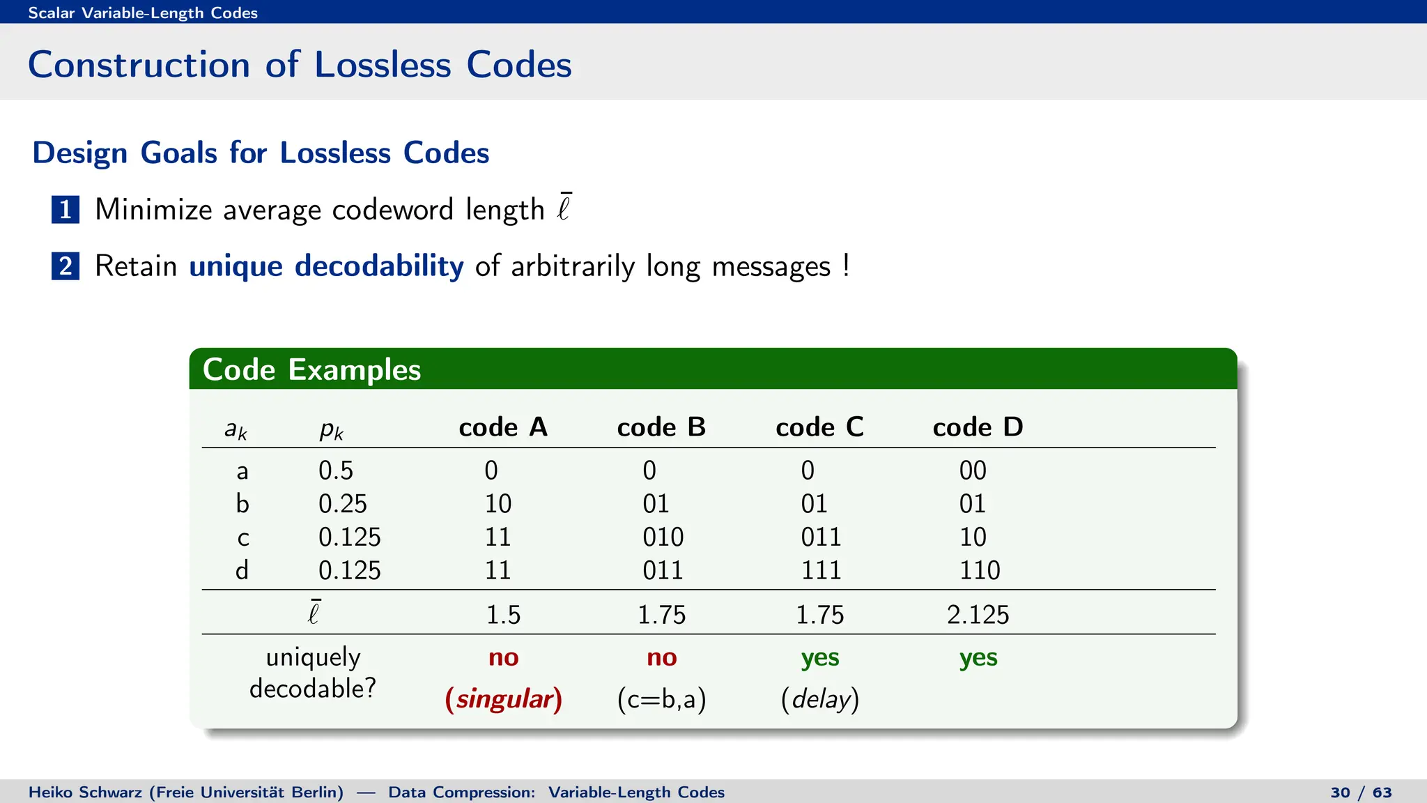
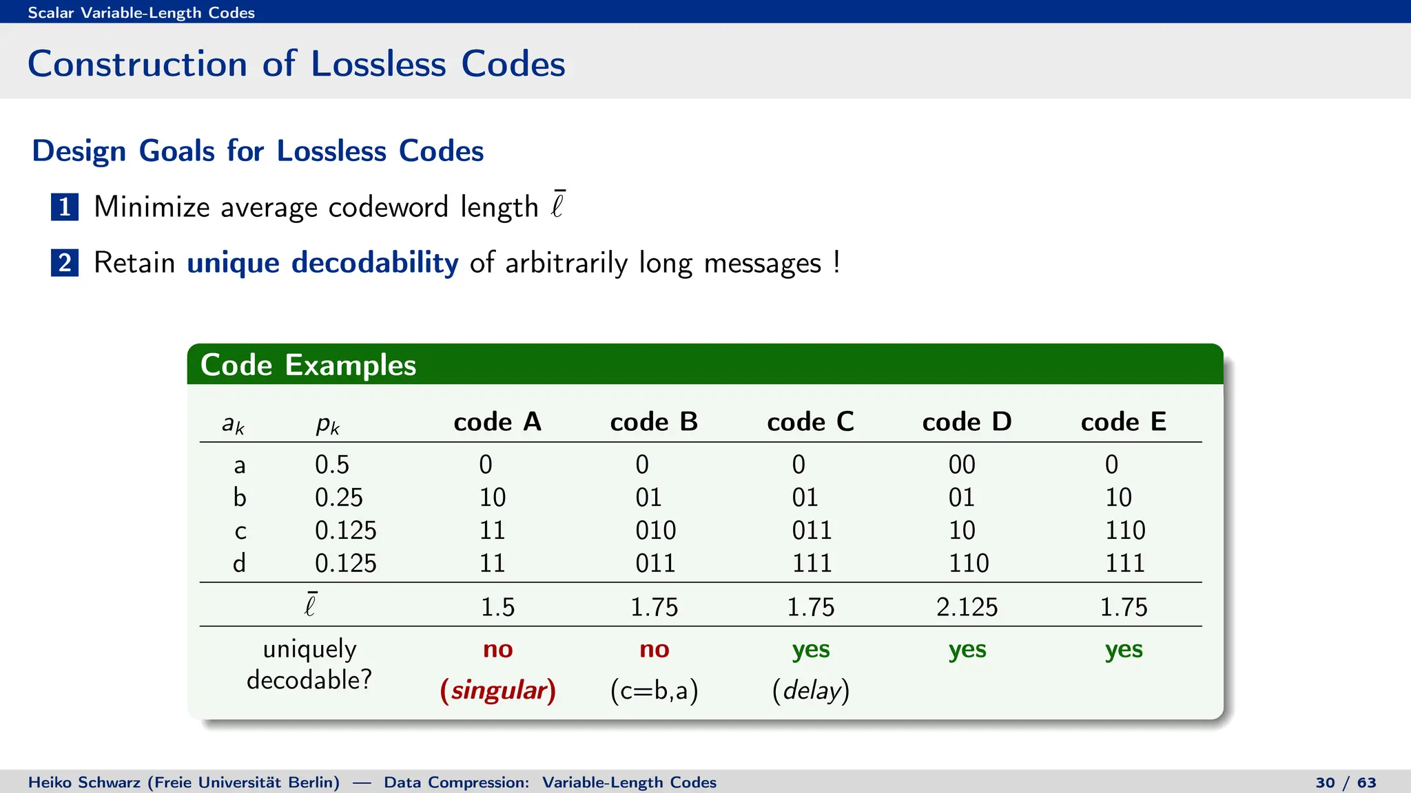
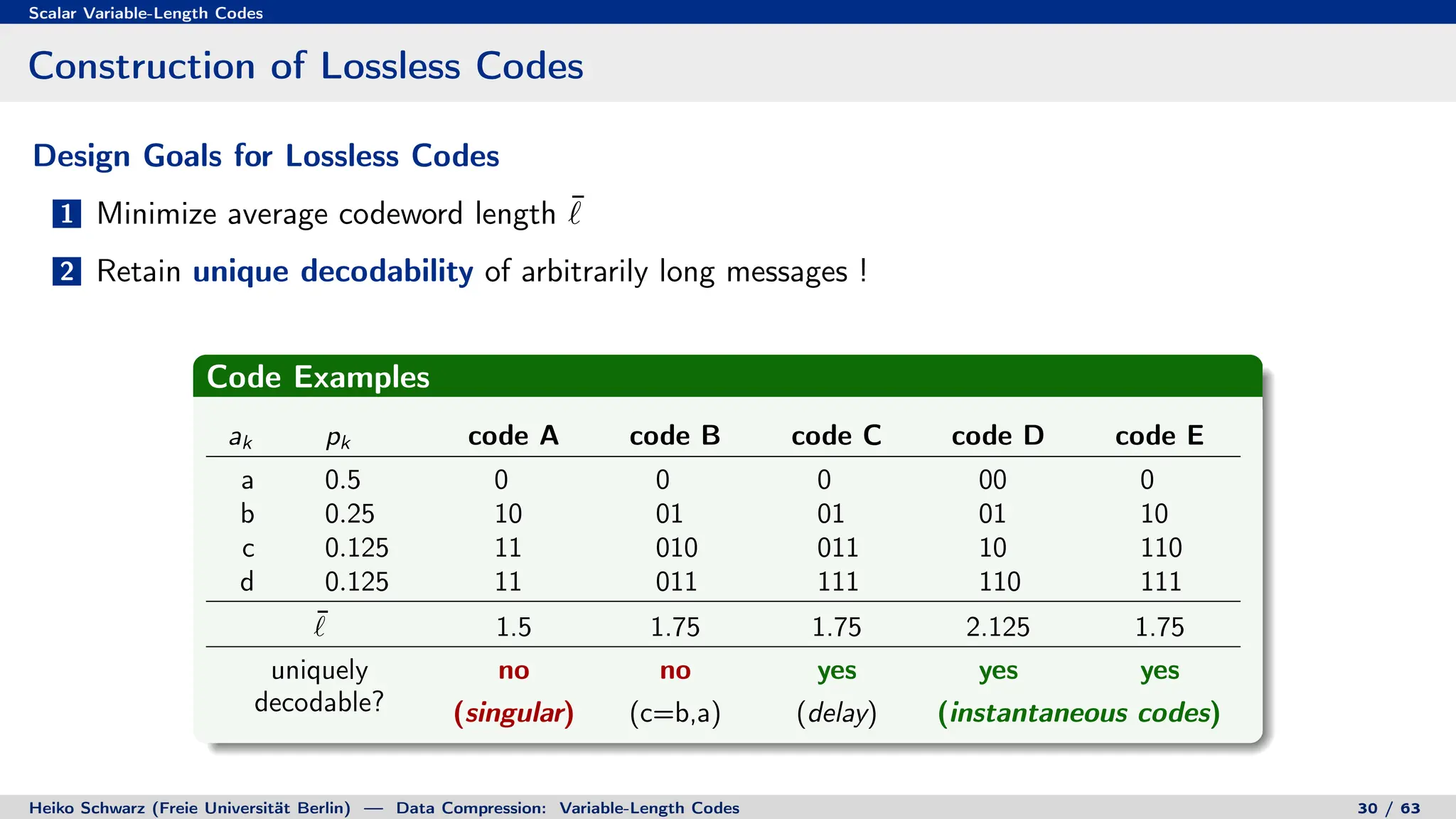
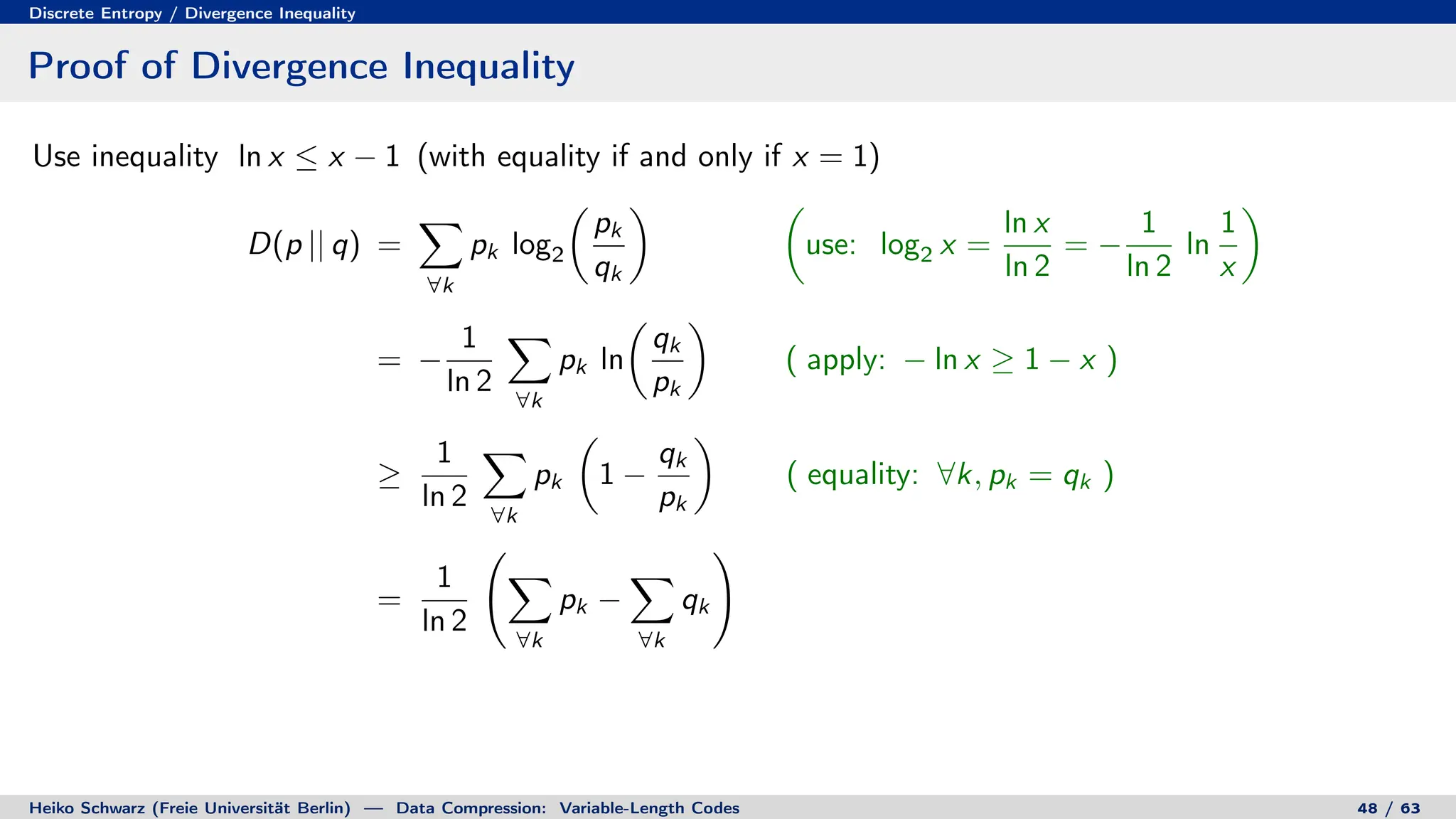
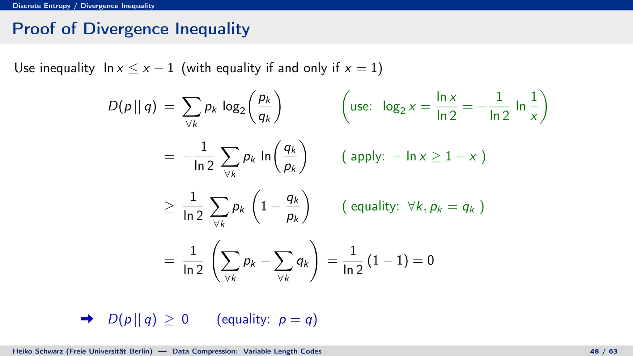
2. Probability theory provides the framework for characterizing information sources and measuring the performance of compression systems using statistical averages.
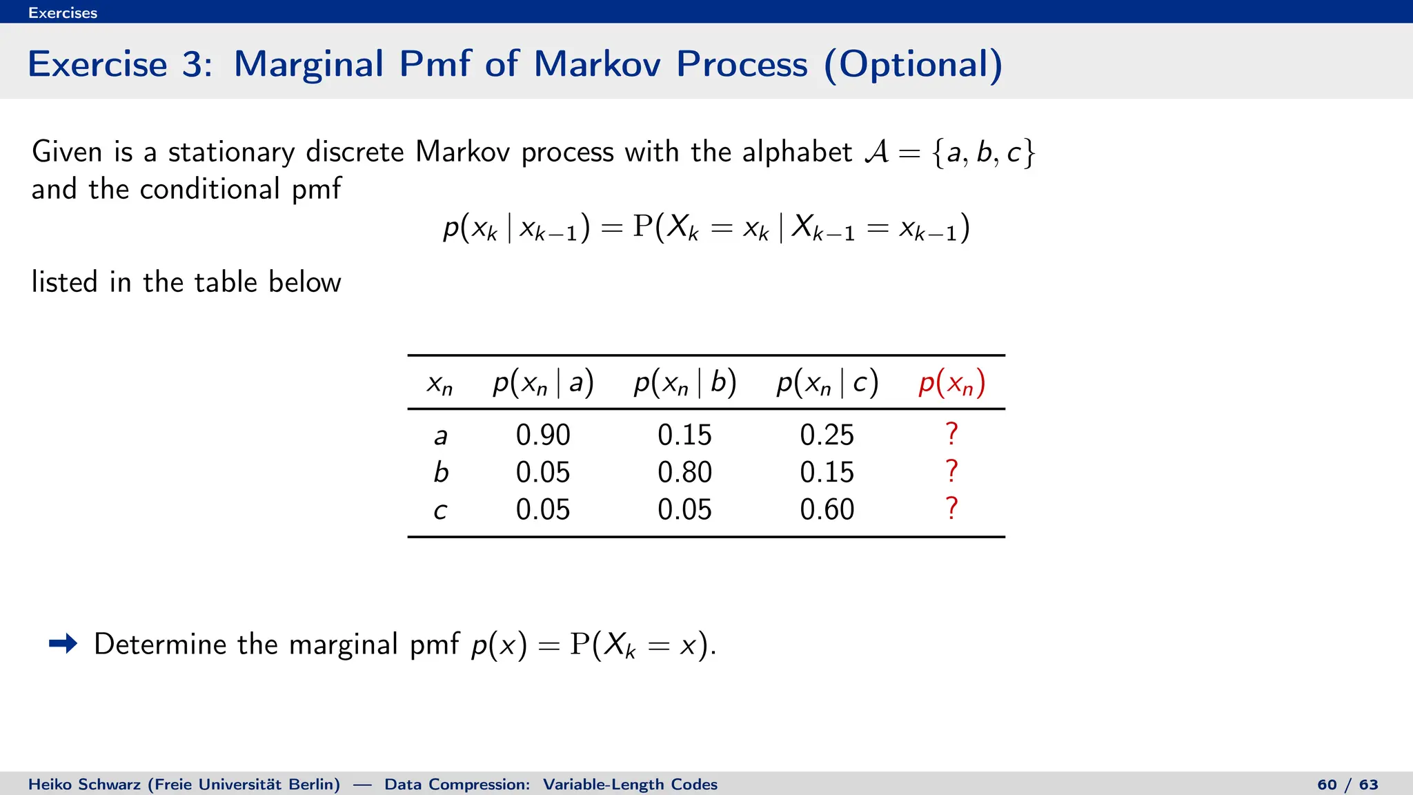
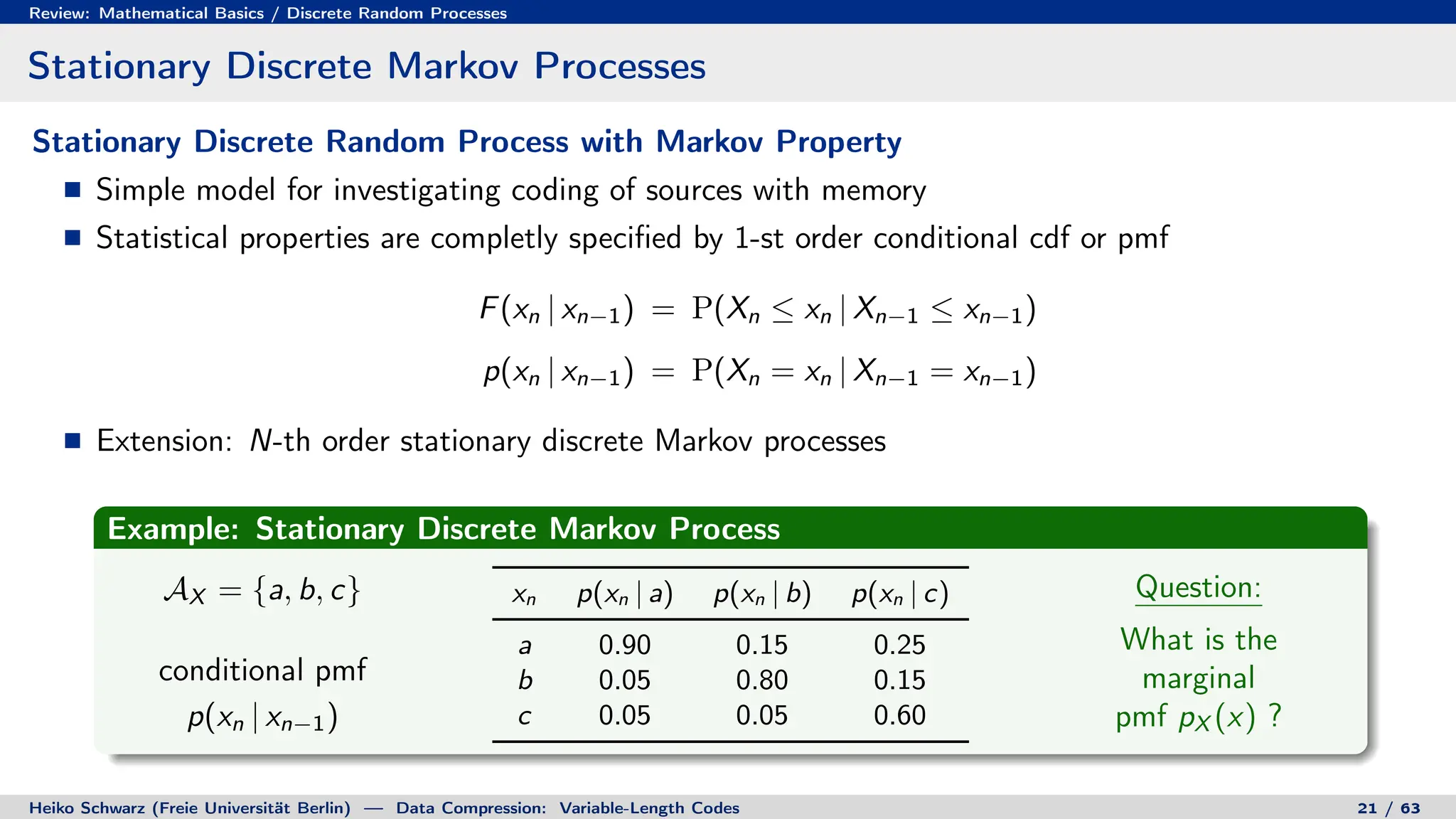
3. Stationary discrete Markov processes are a simple model for investigating coding of sources with memory, defined by their conditional probability distributions.


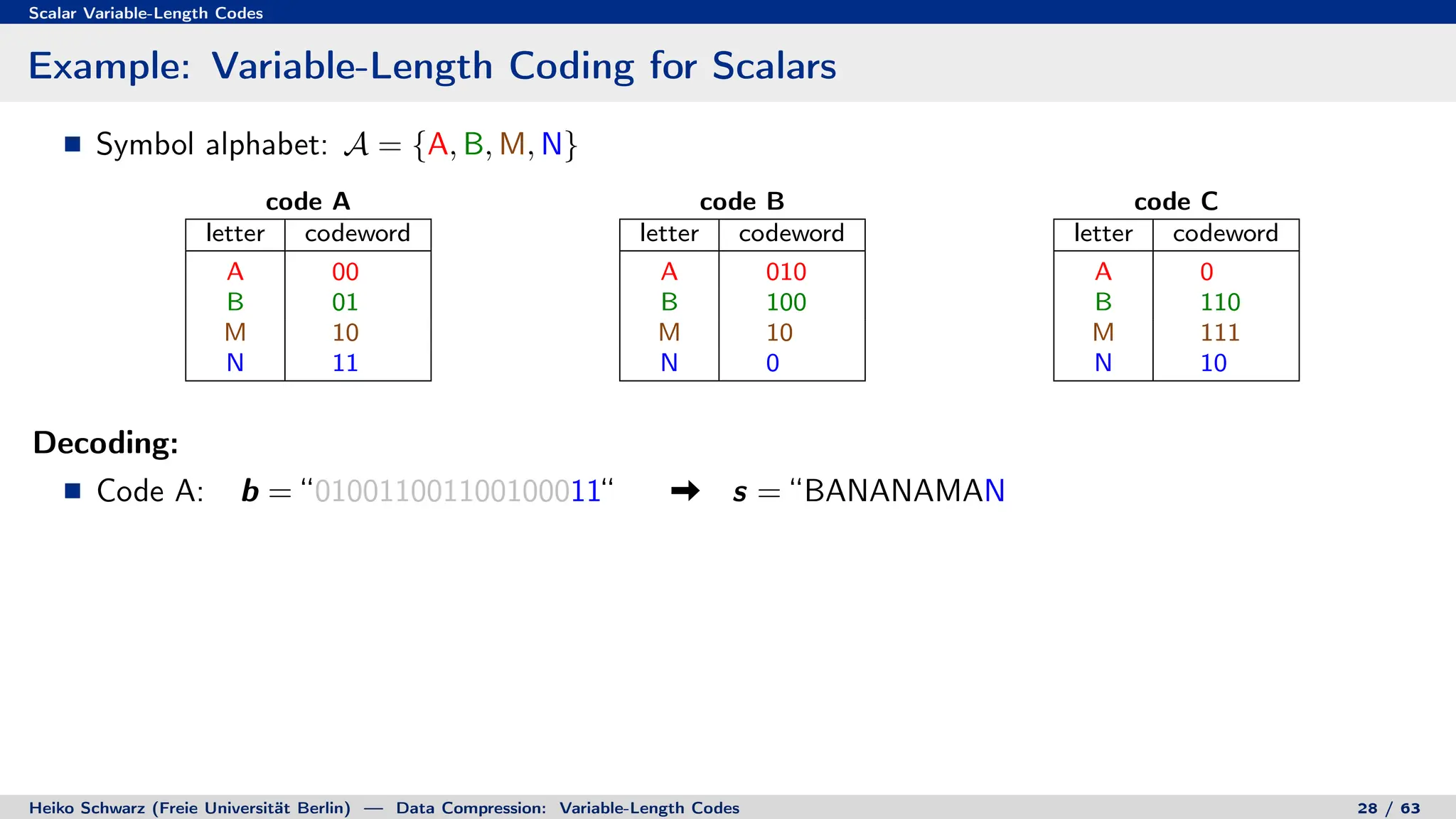

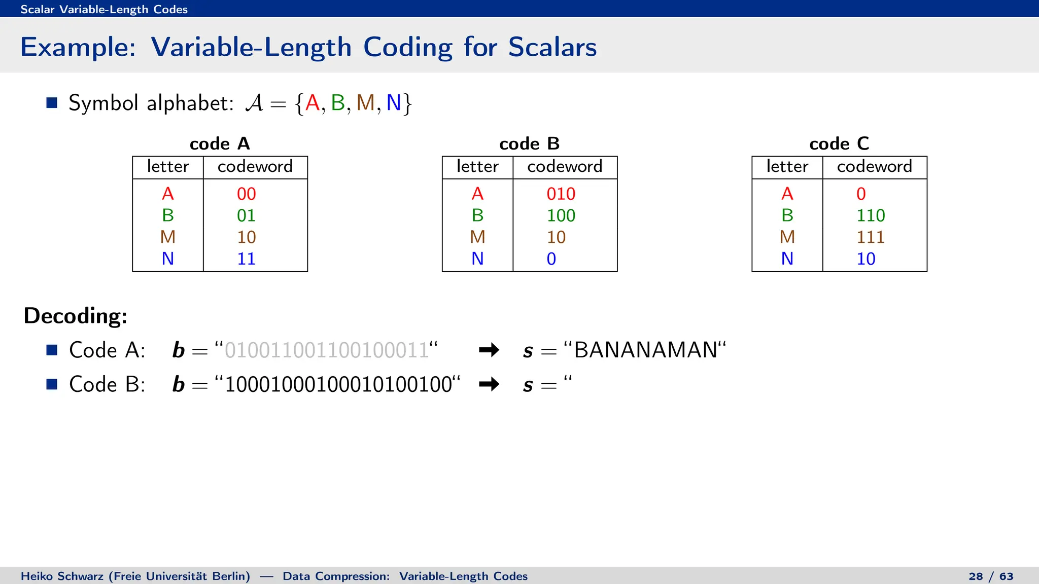
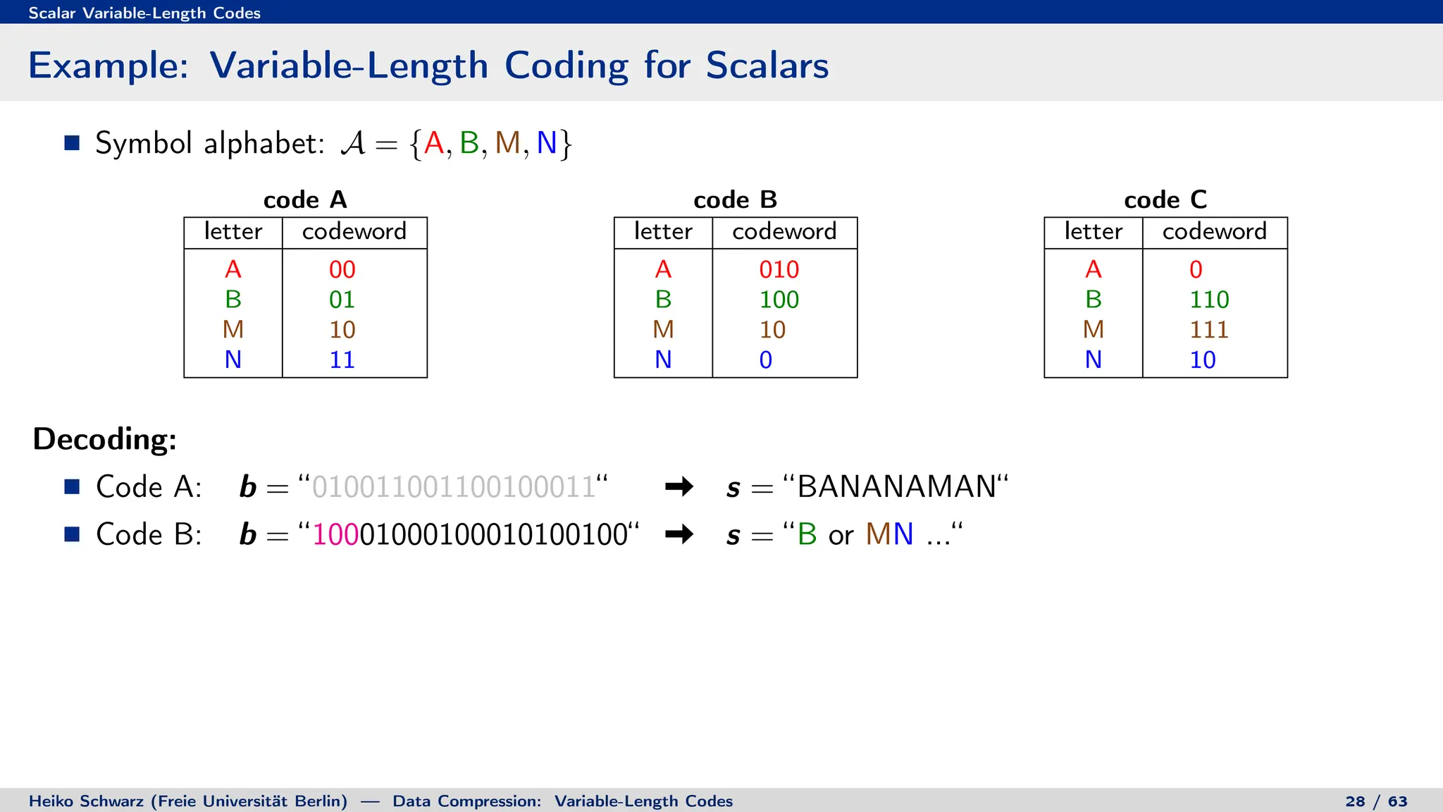


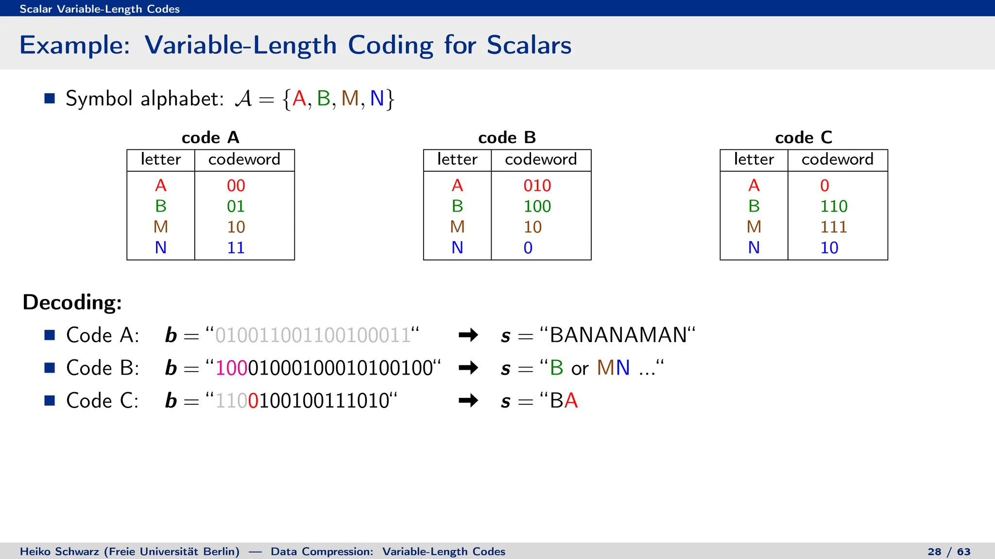


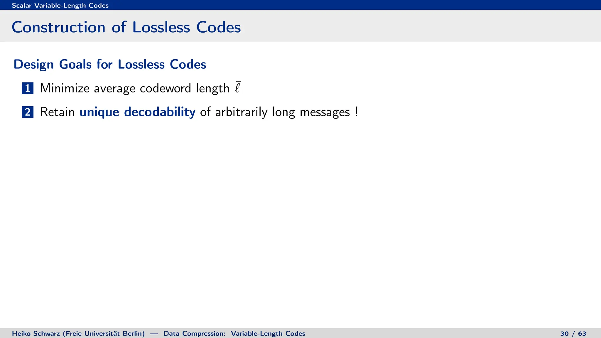

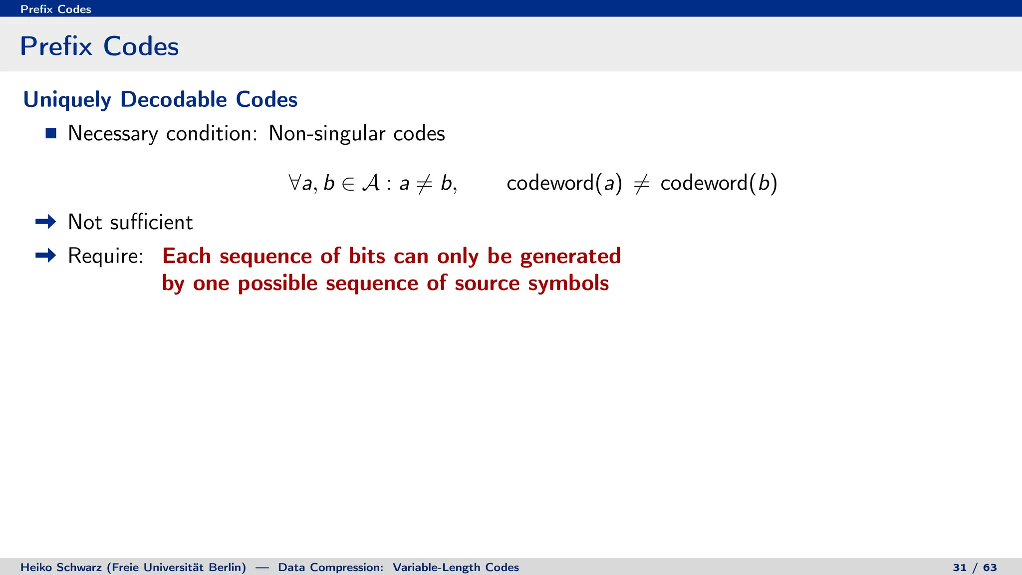
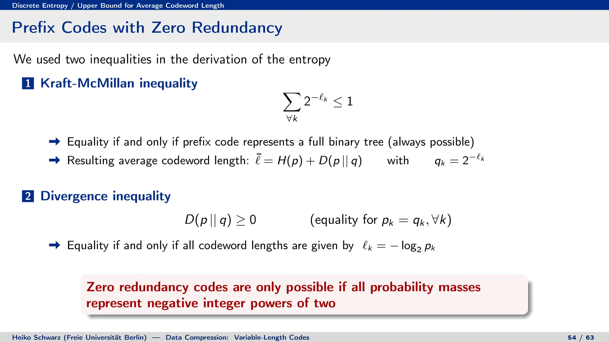
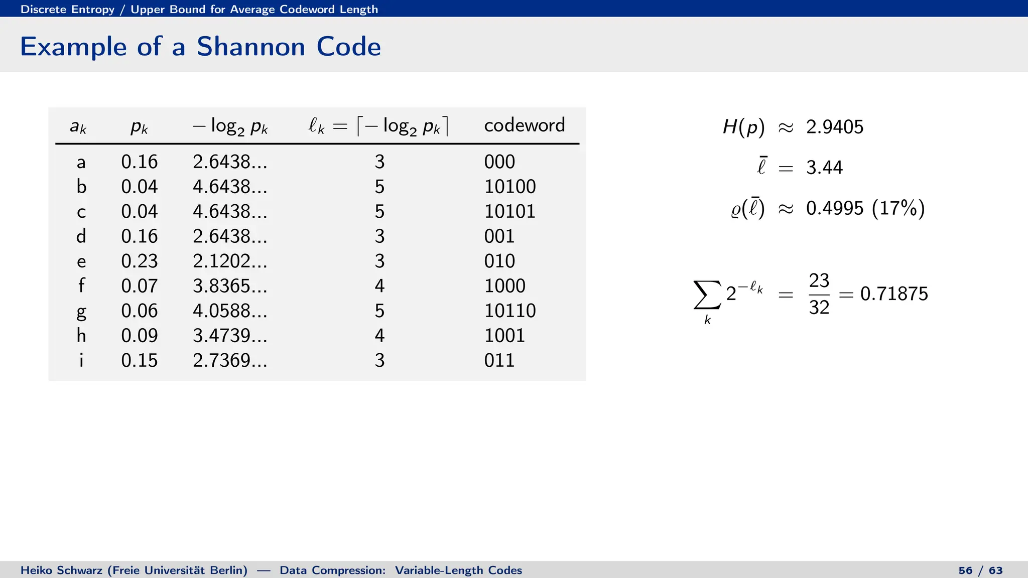
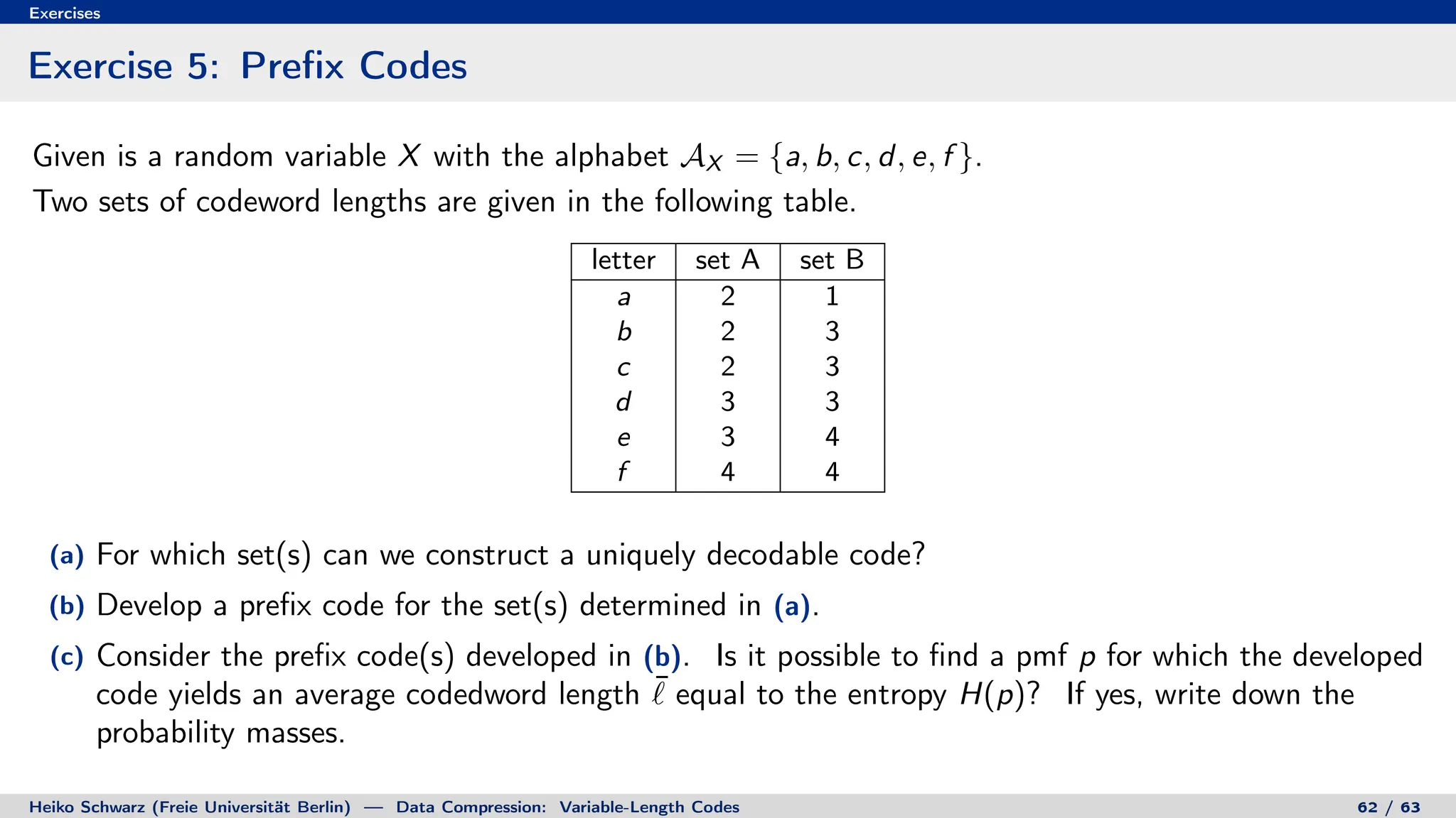
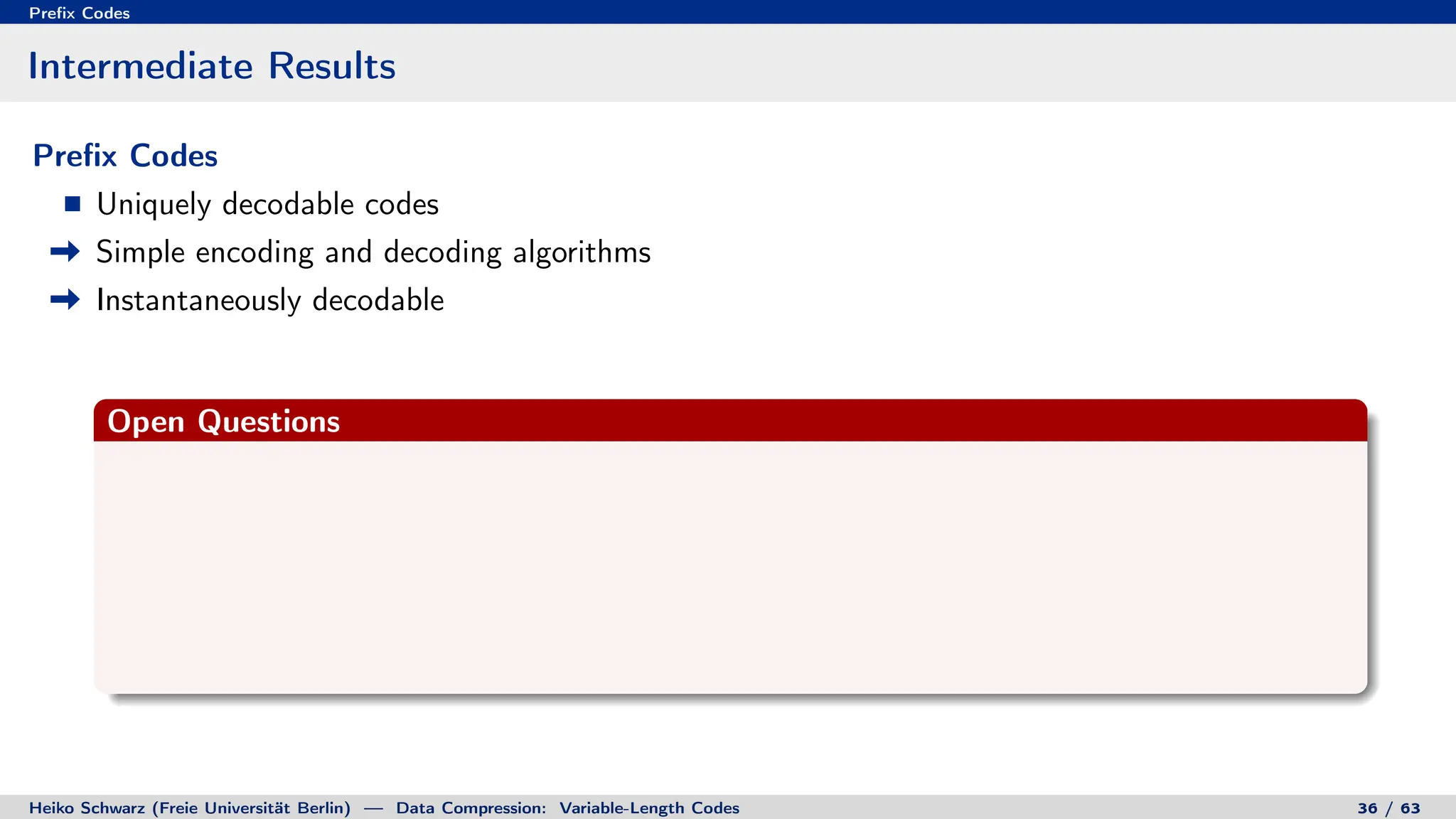
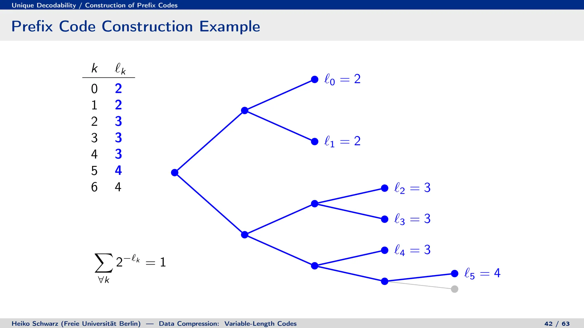
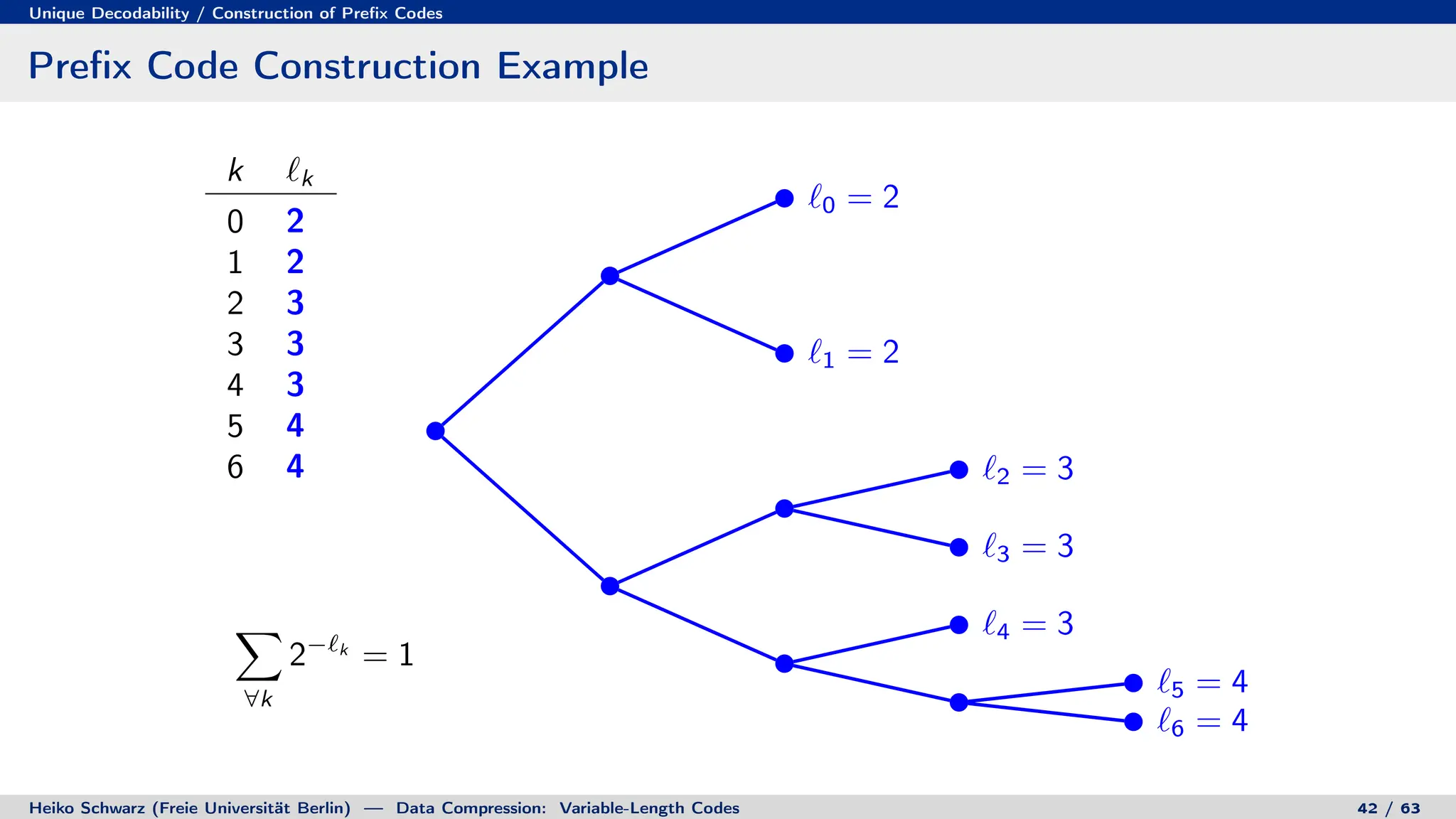
![Prefix Codes
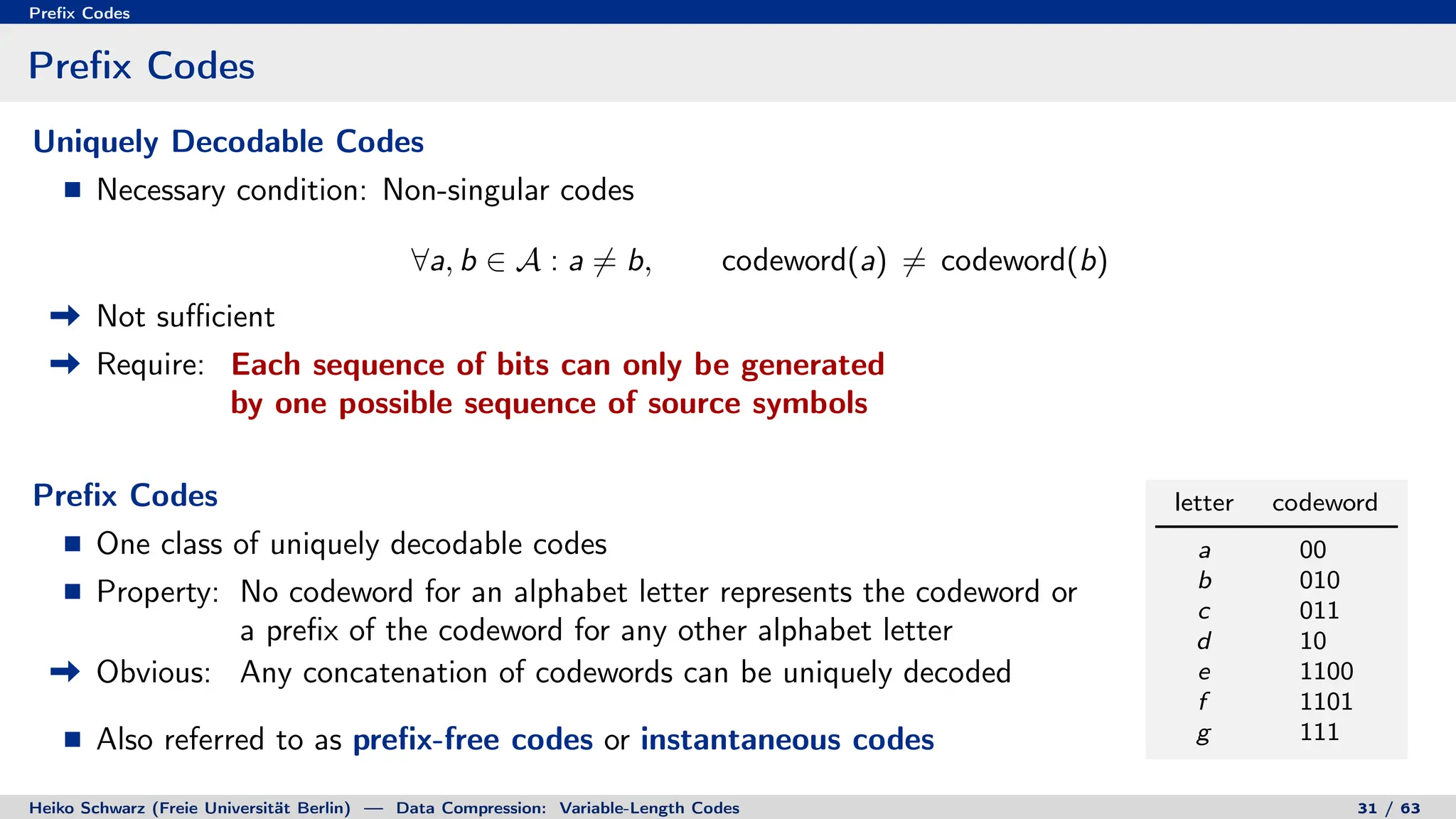
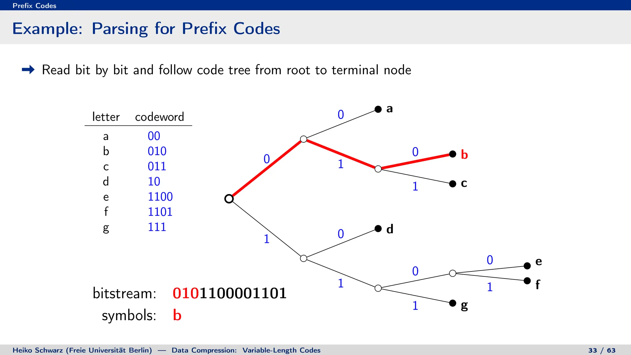
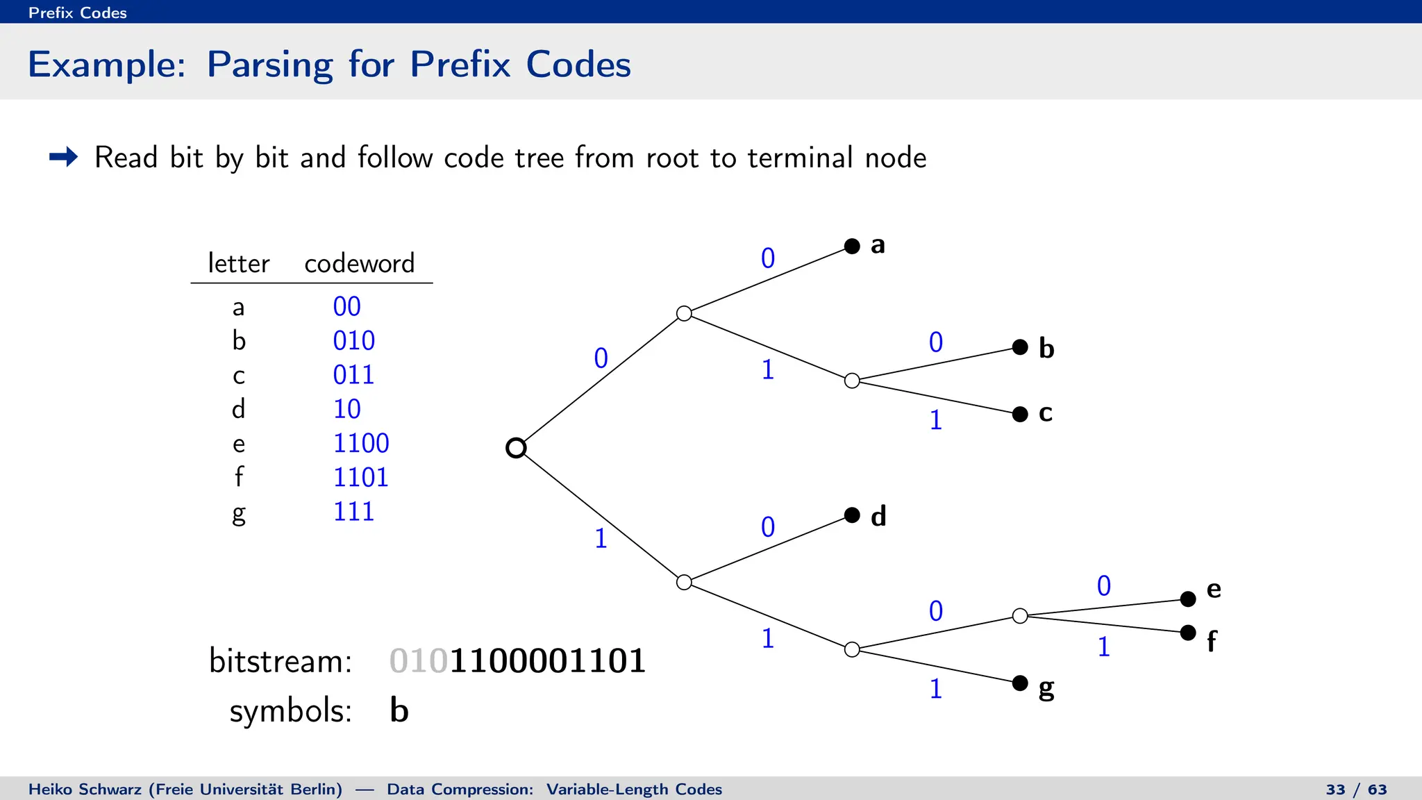
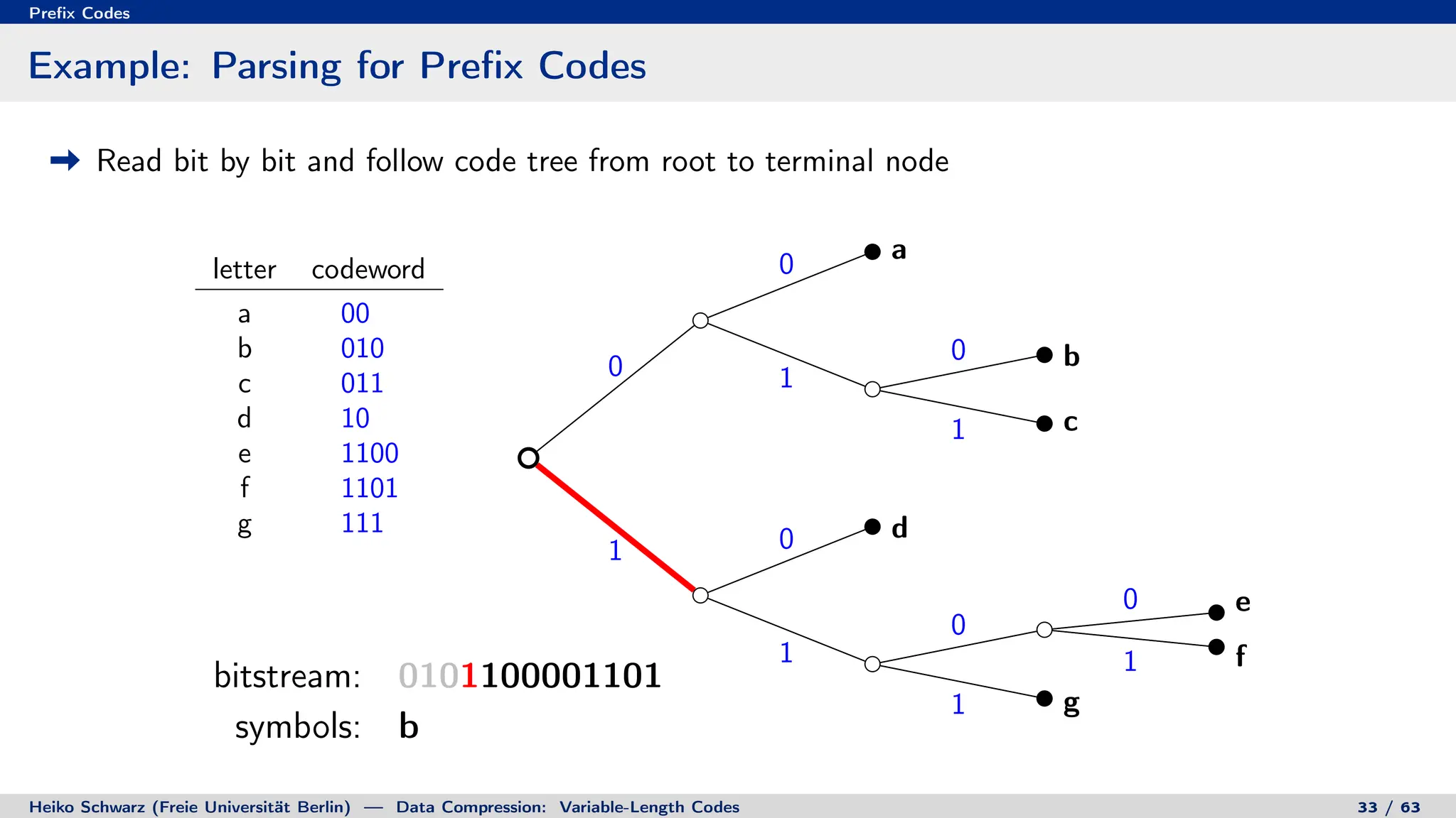
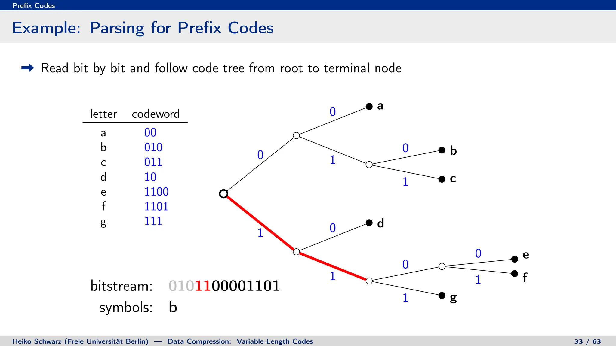
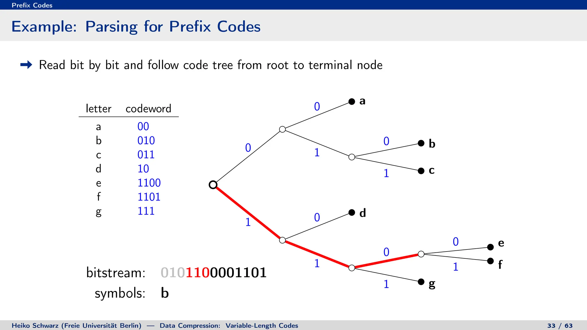
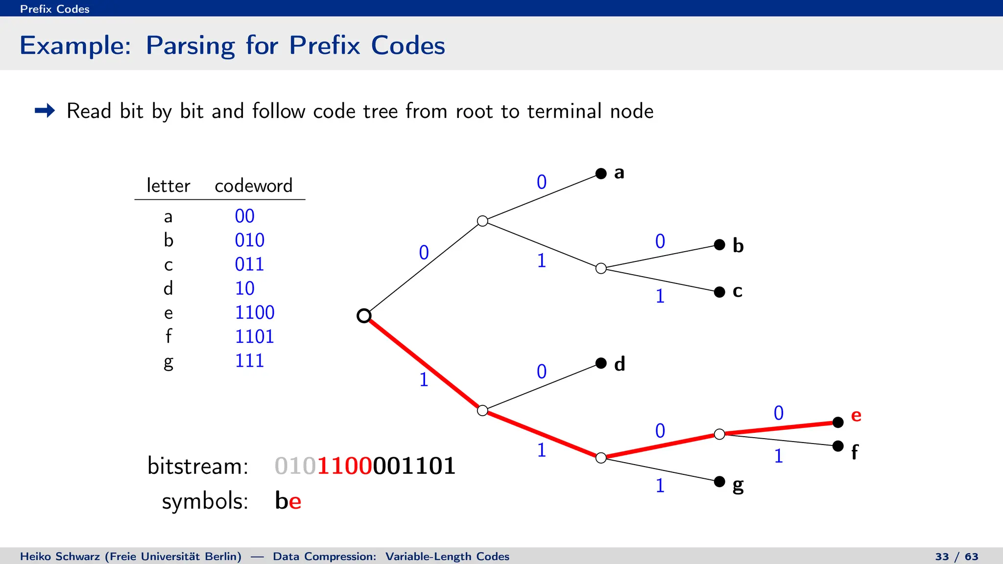
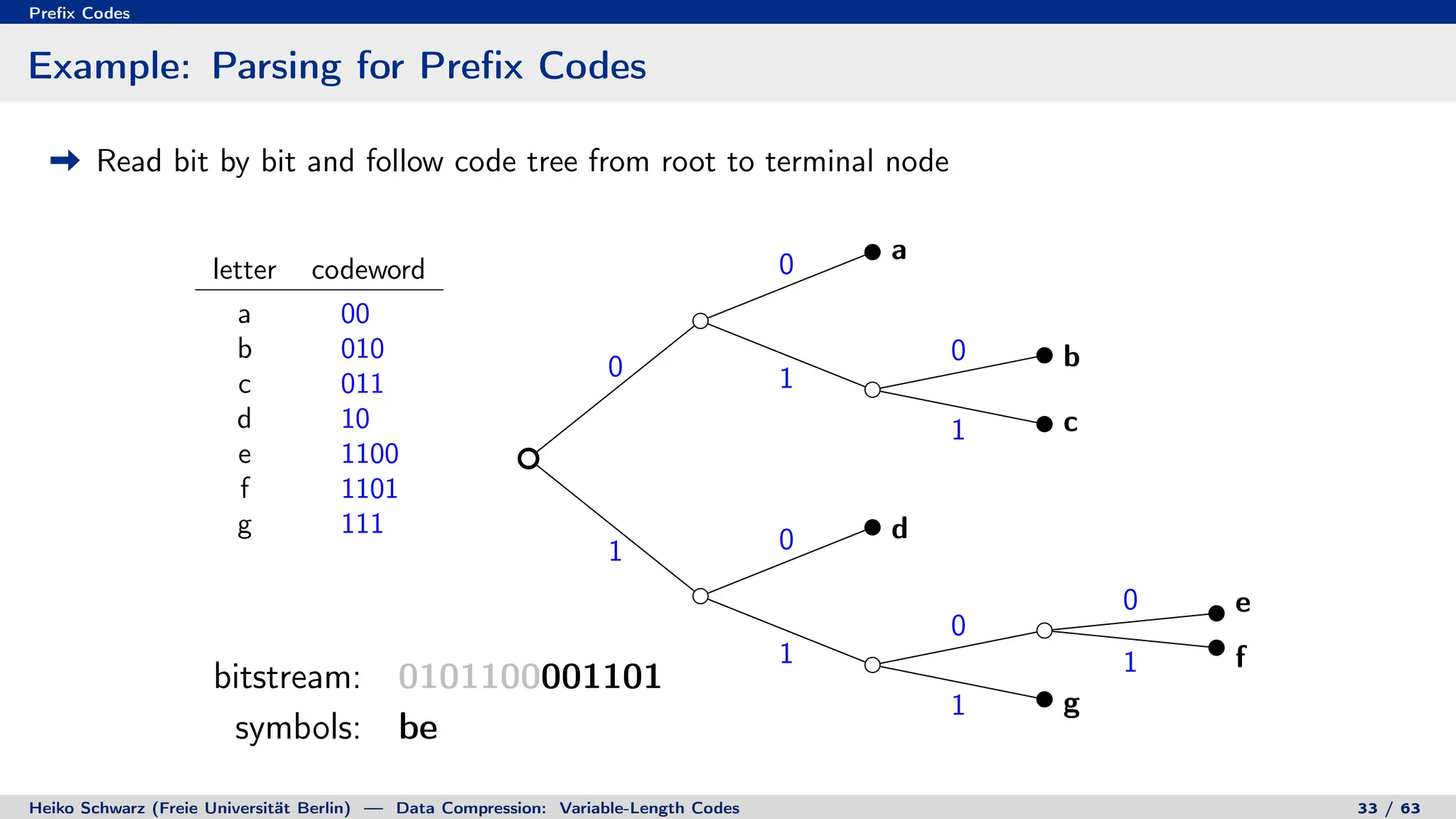
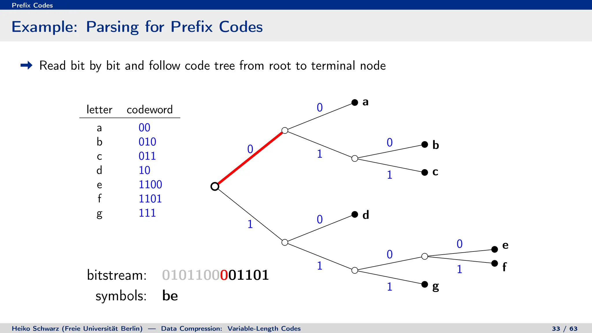
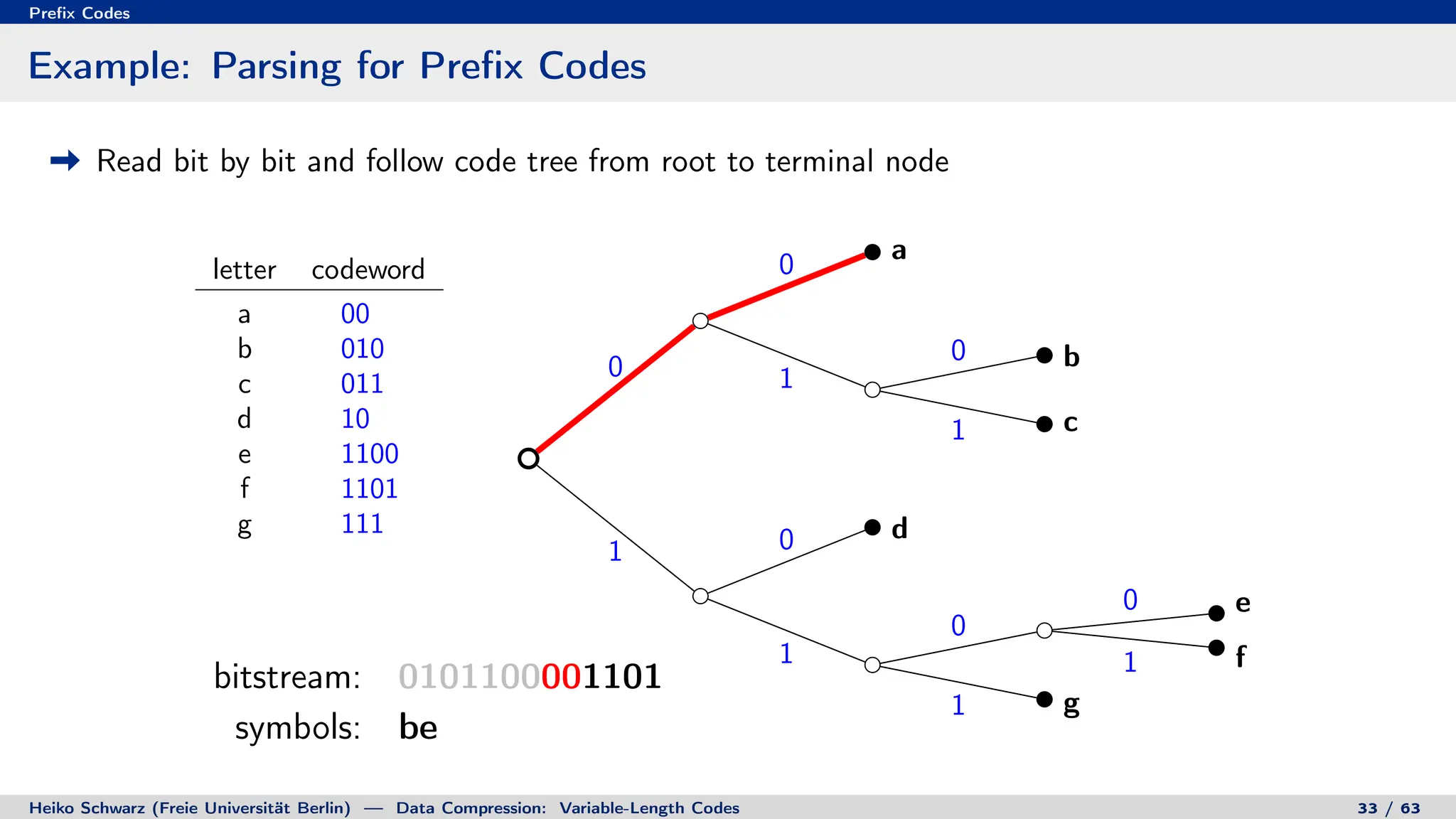
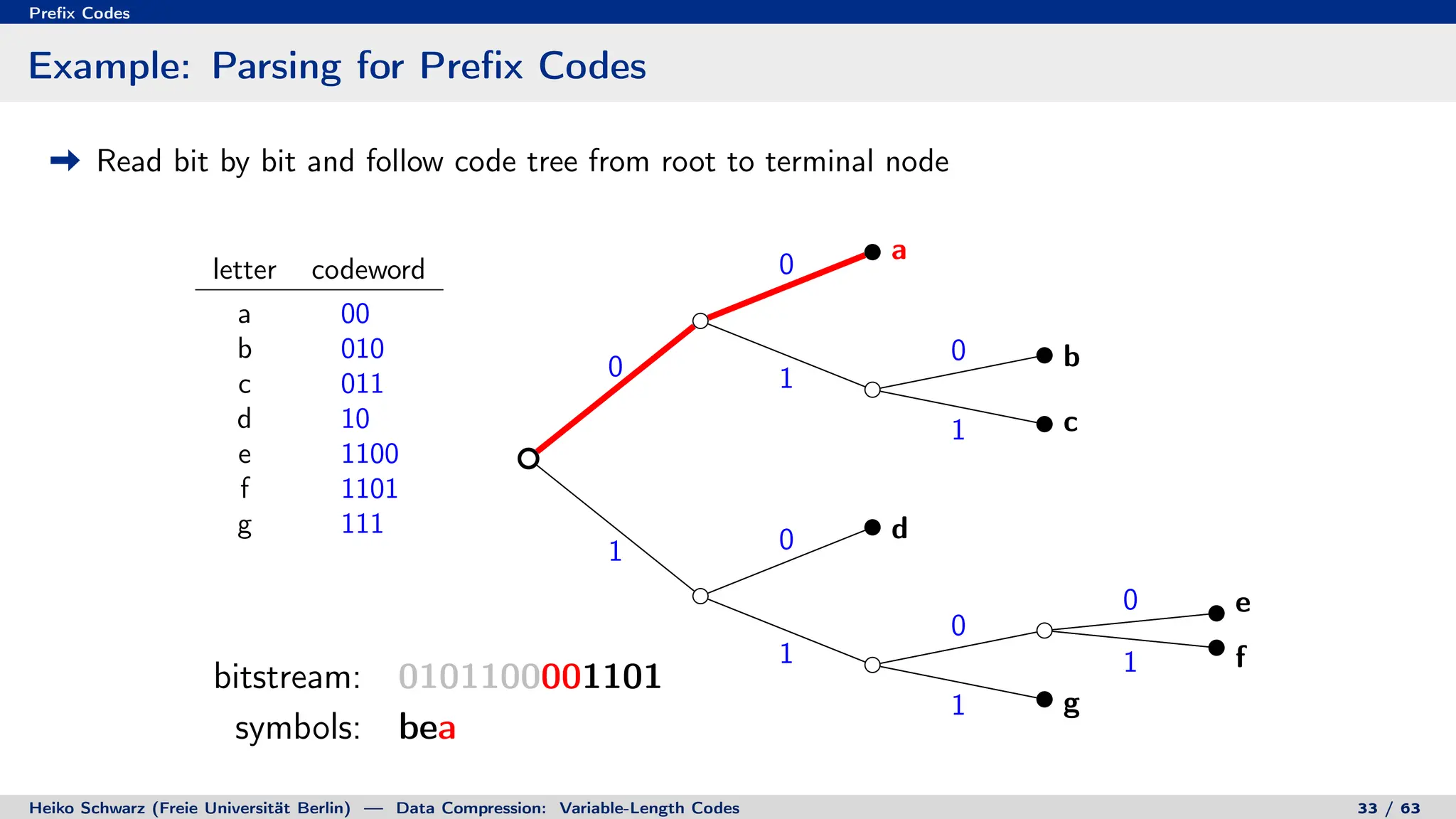
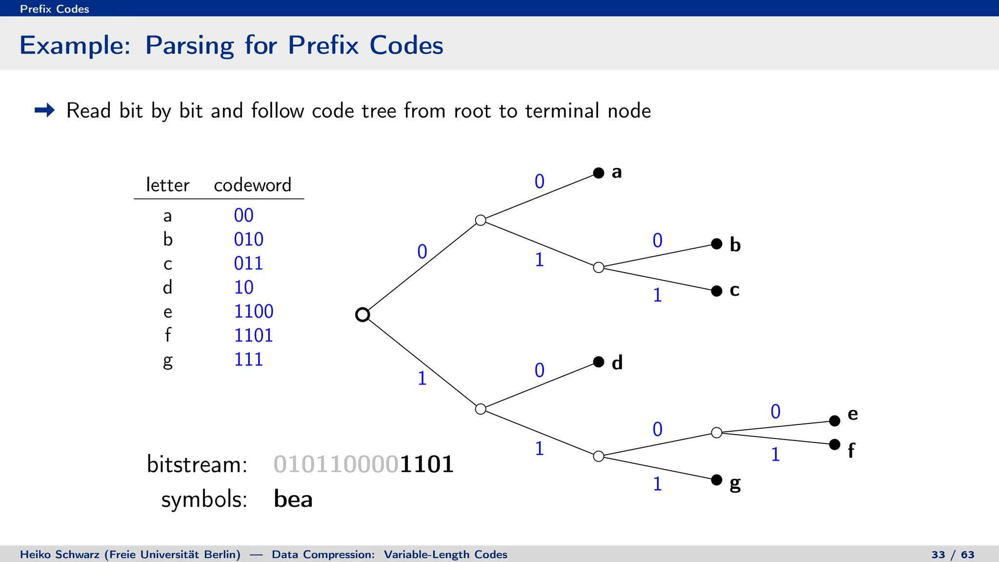
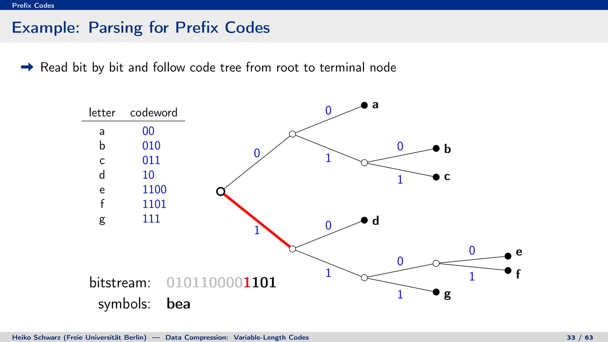
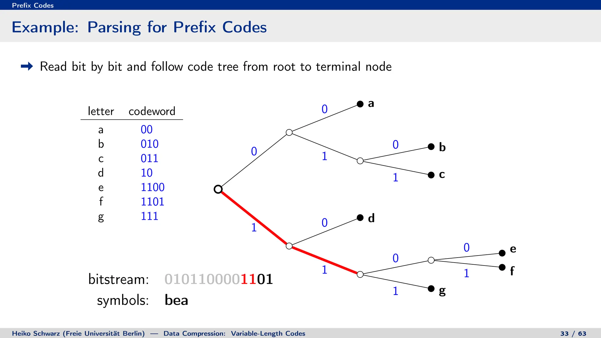
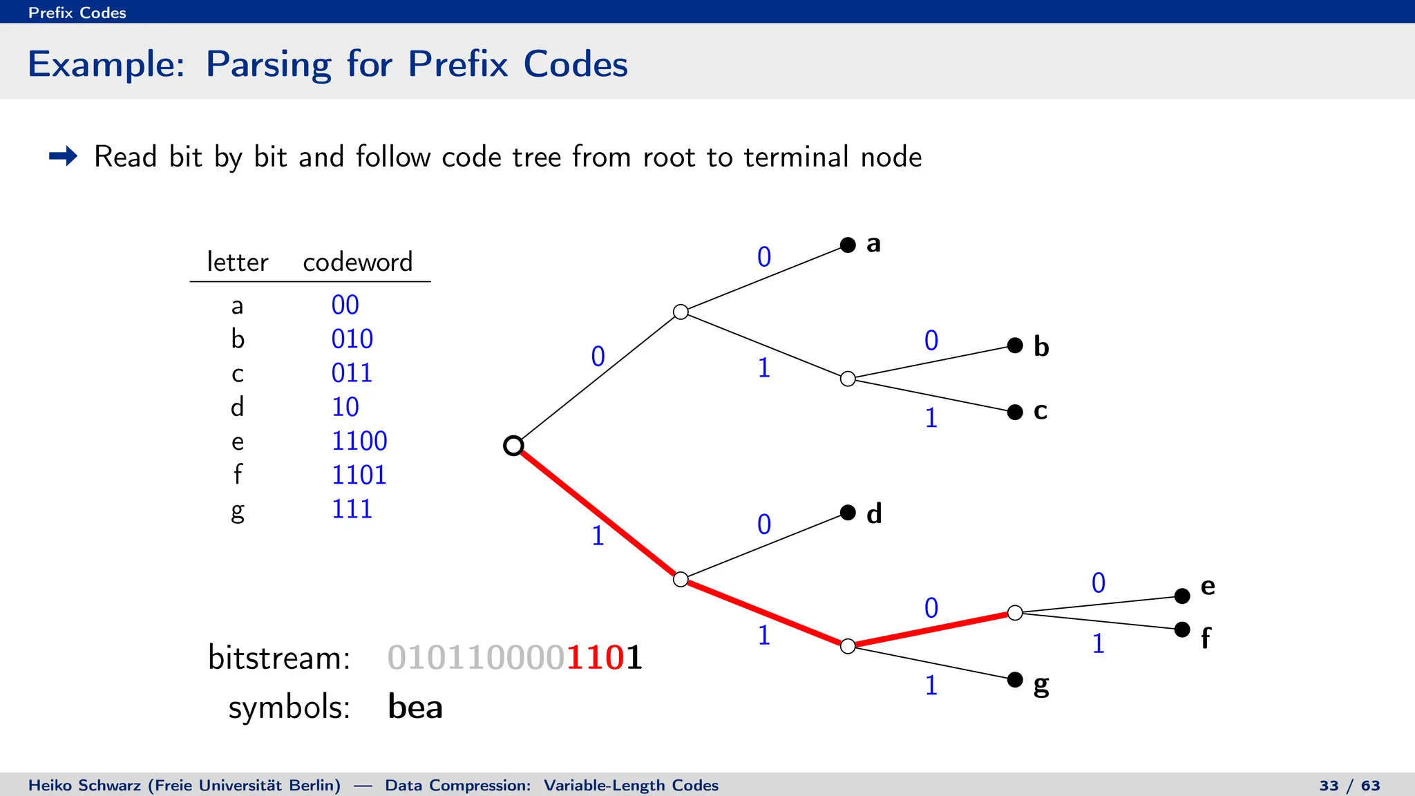
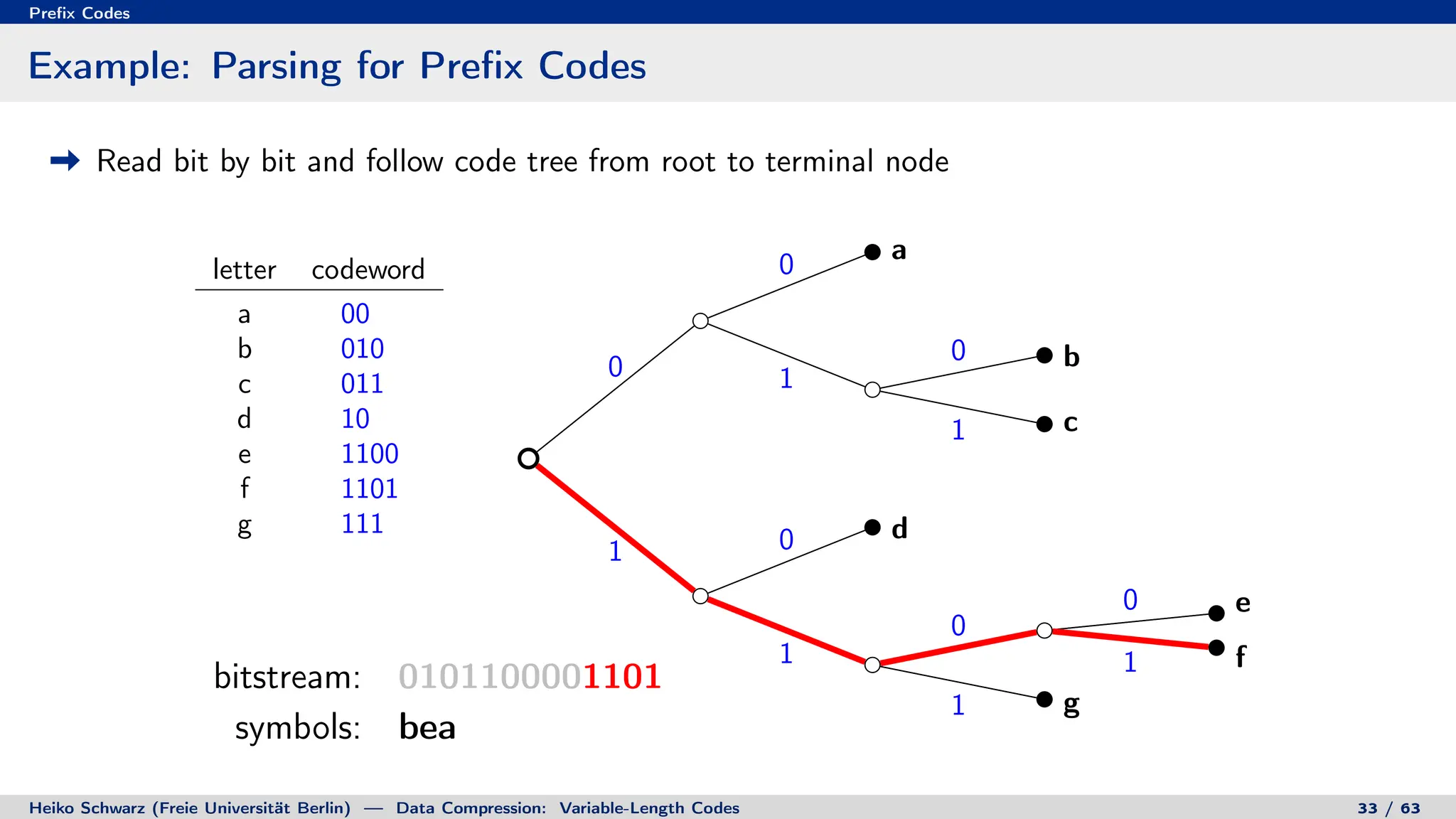
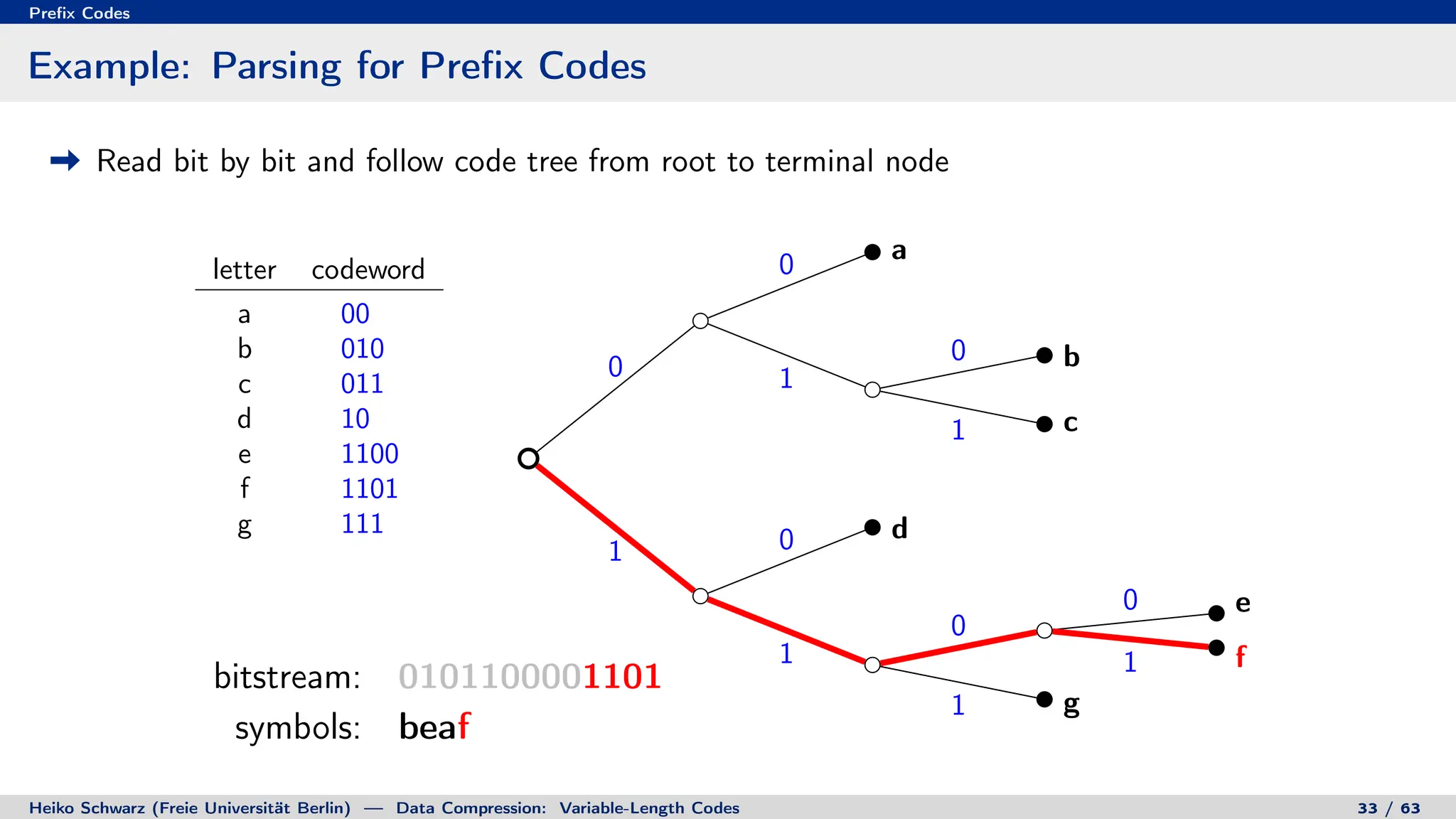
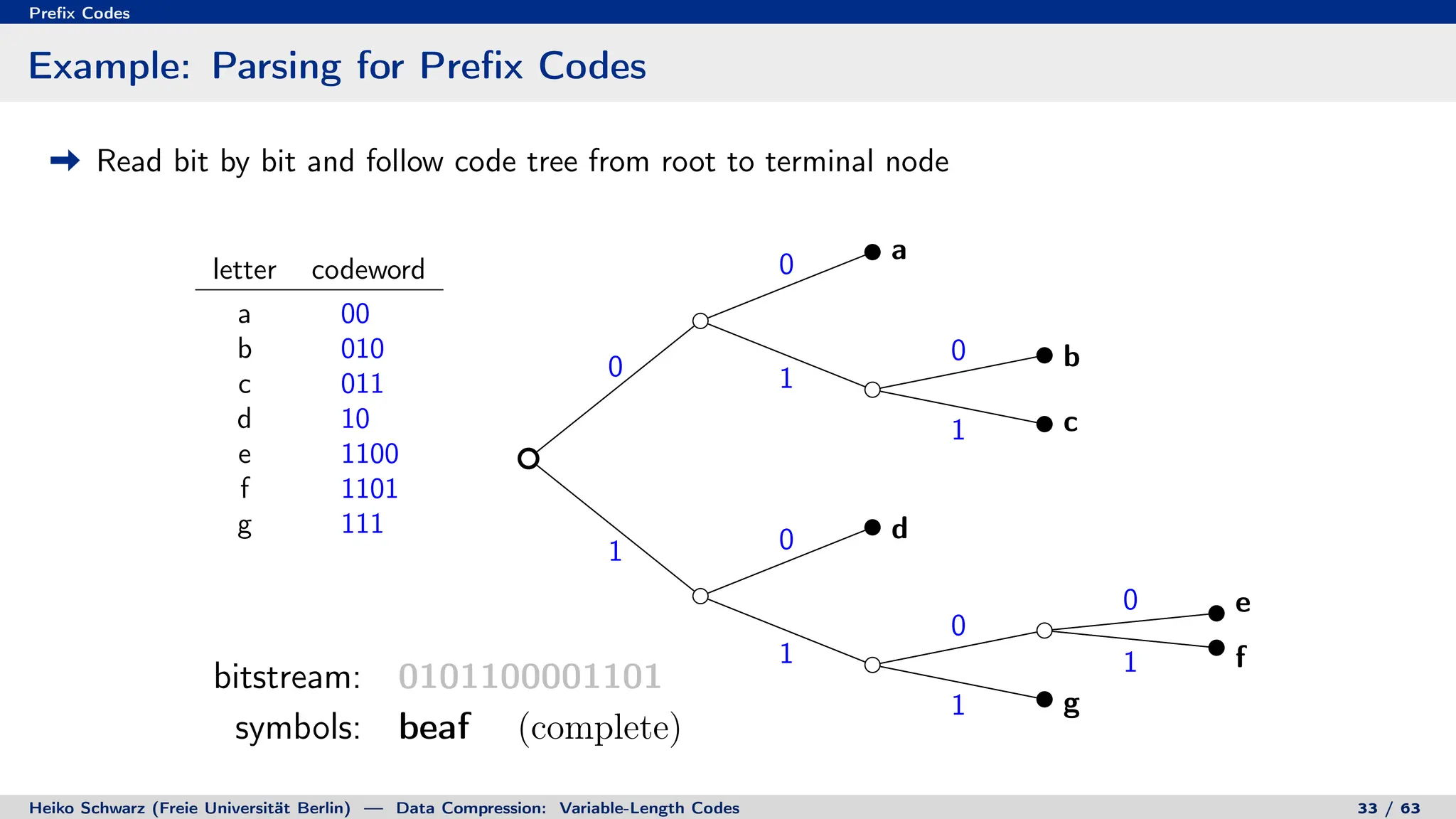
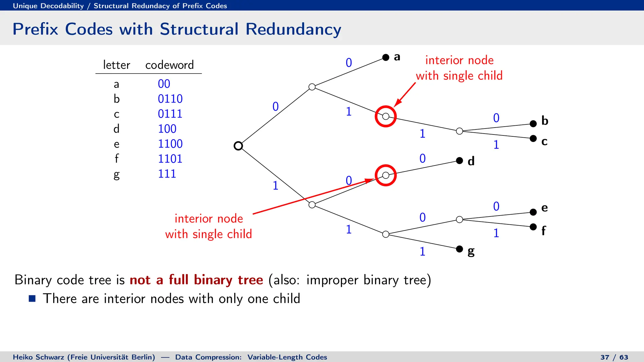
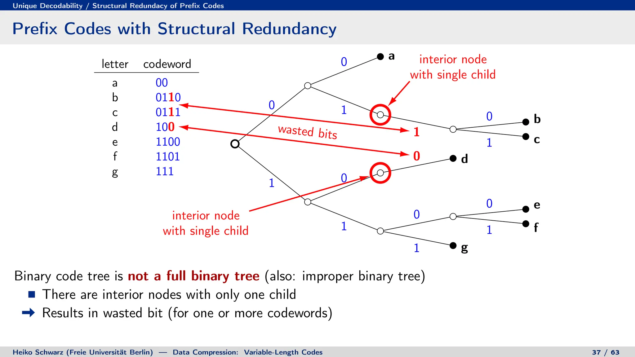
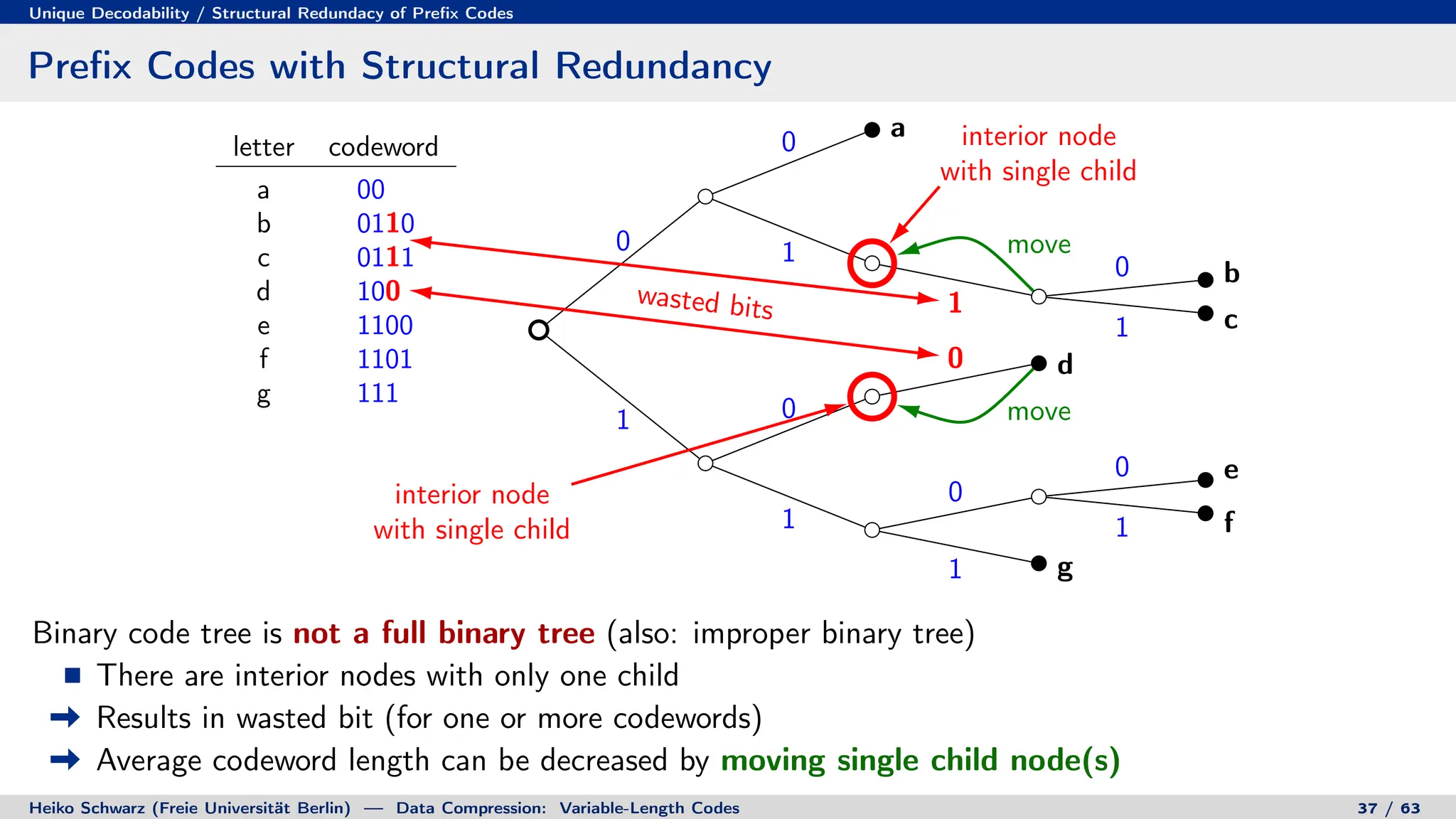
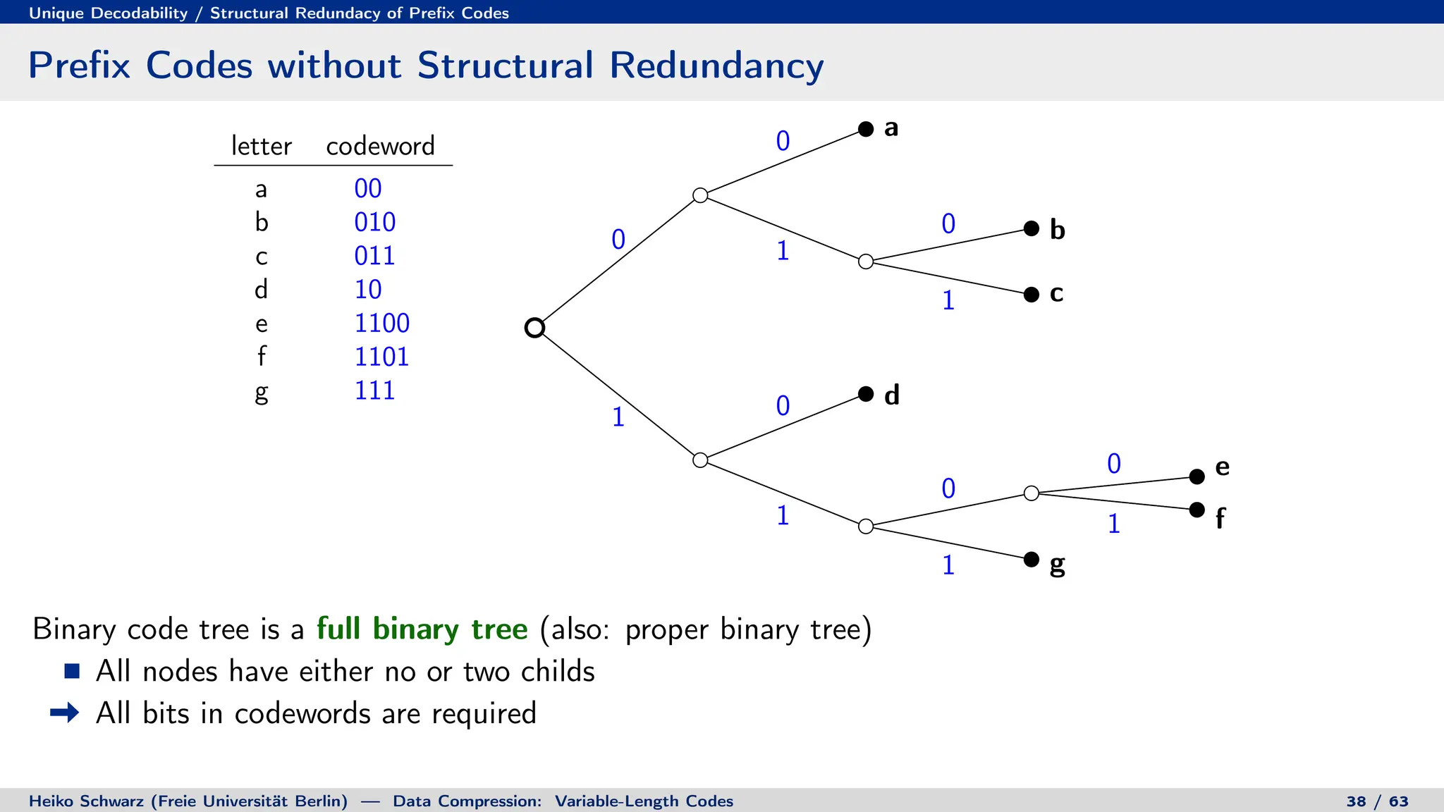
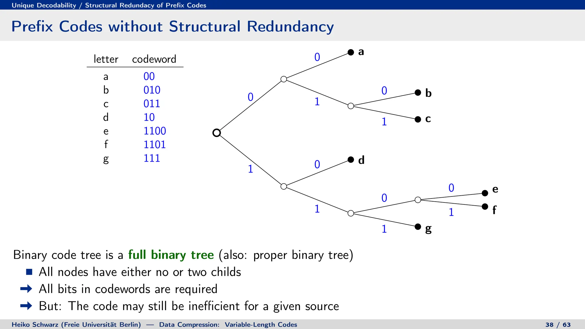
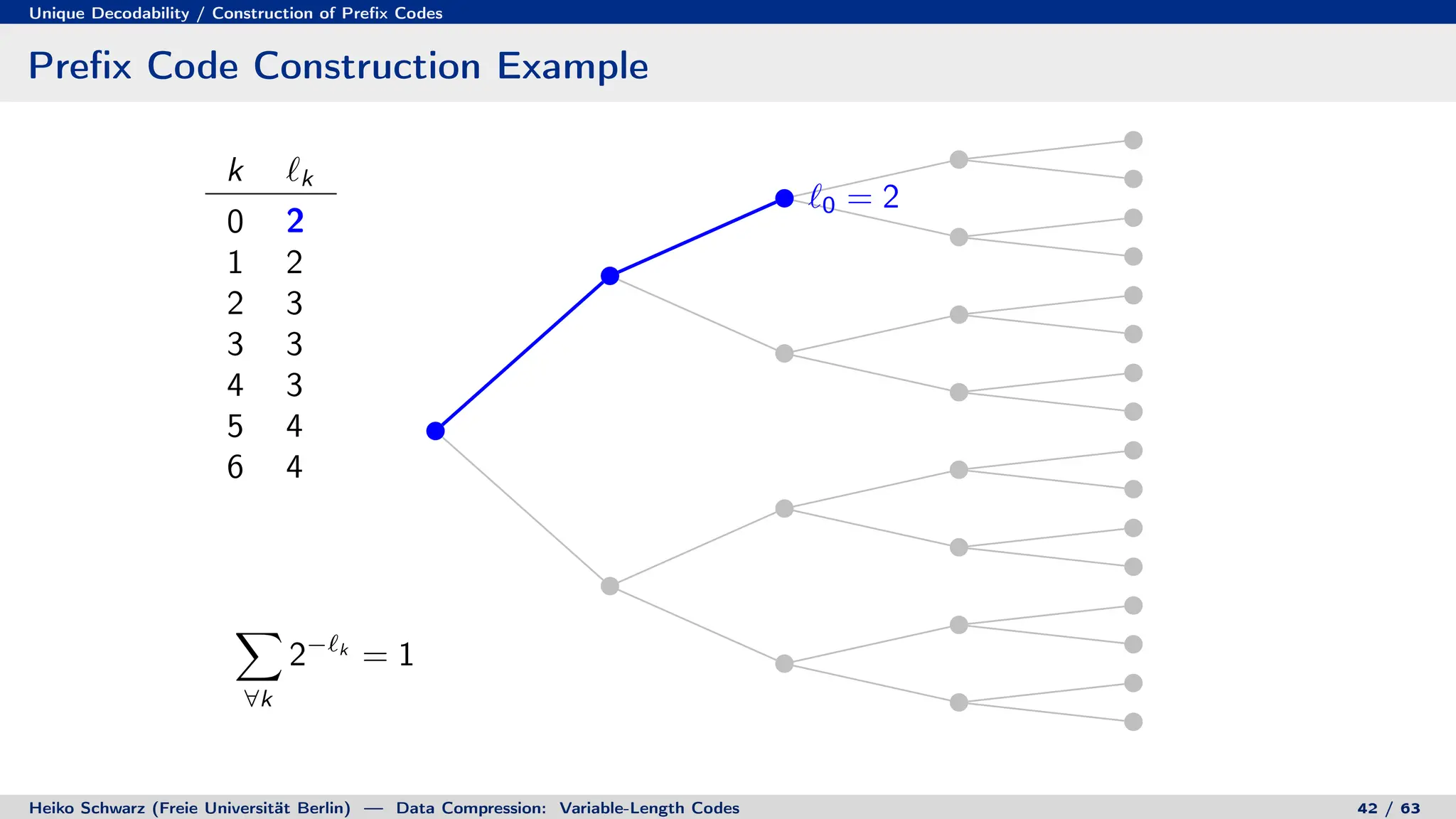
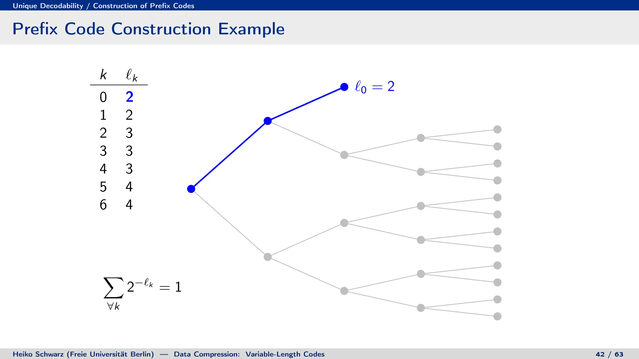
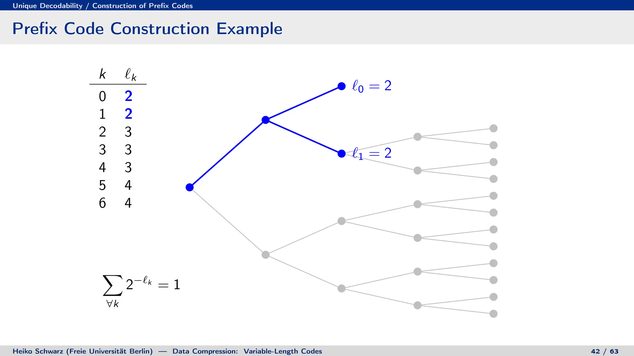
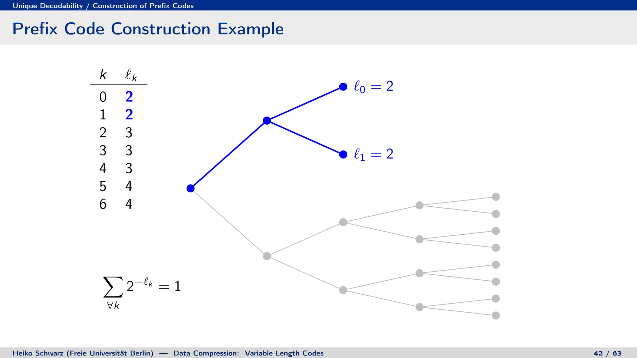
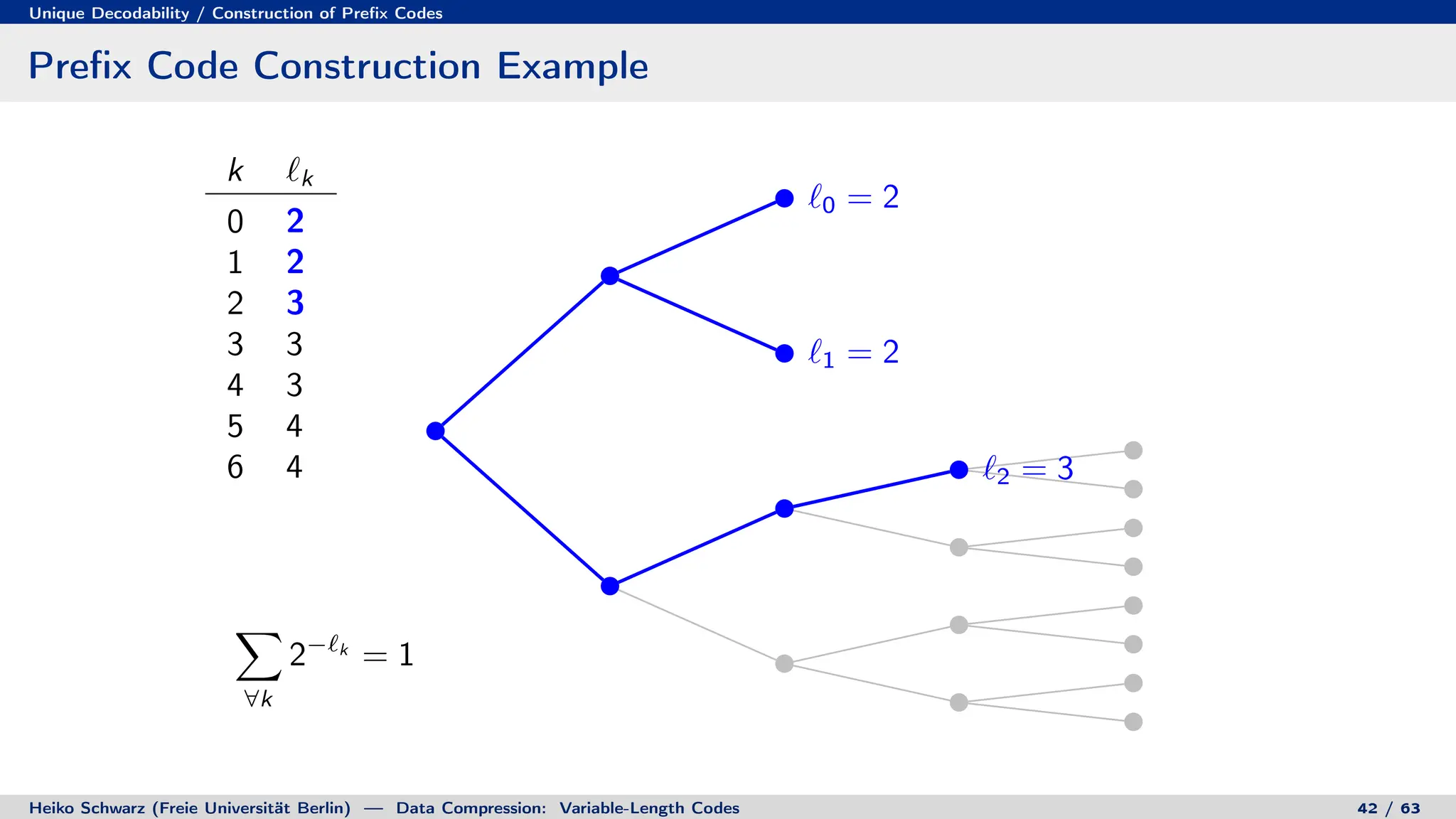
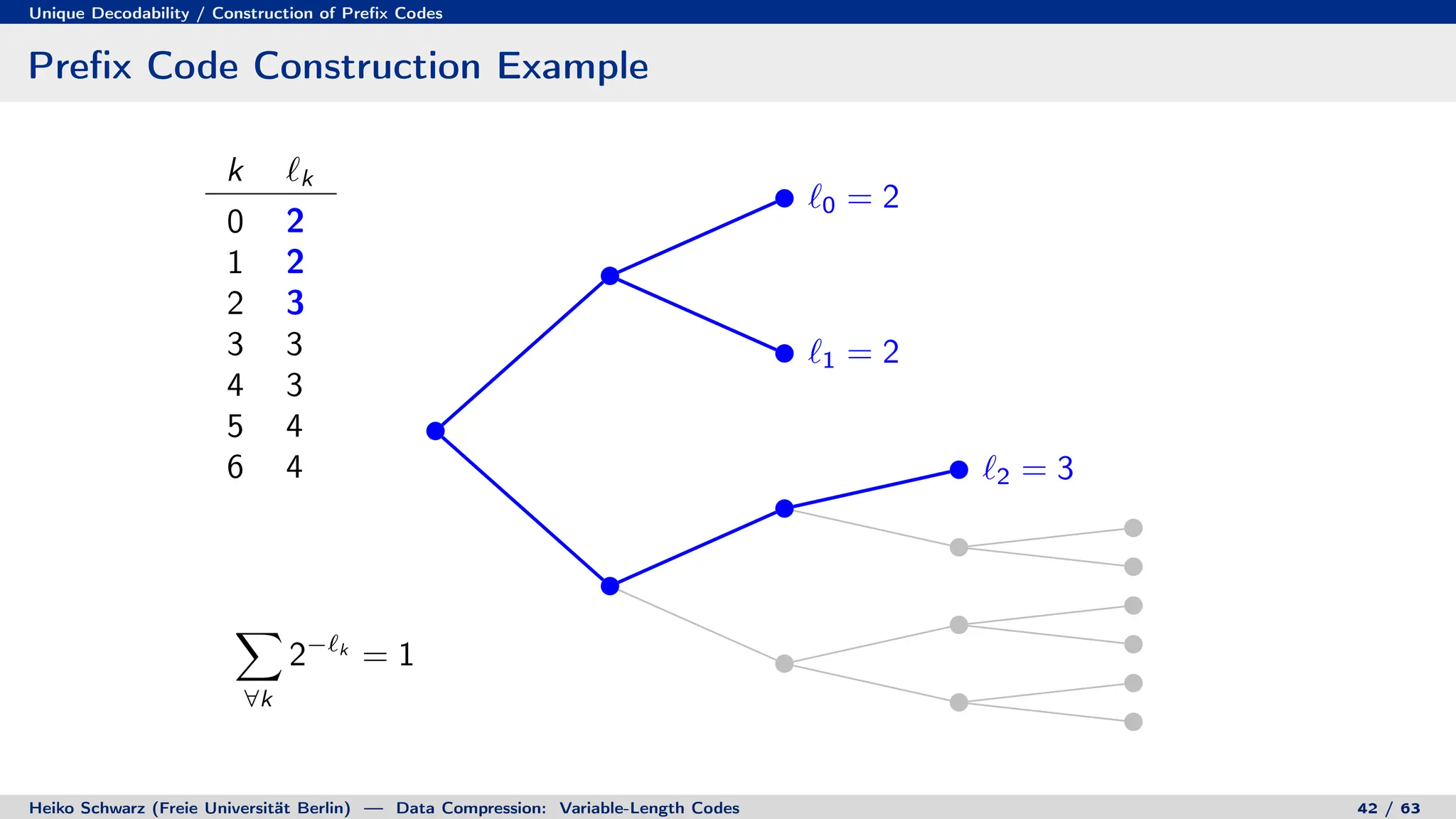
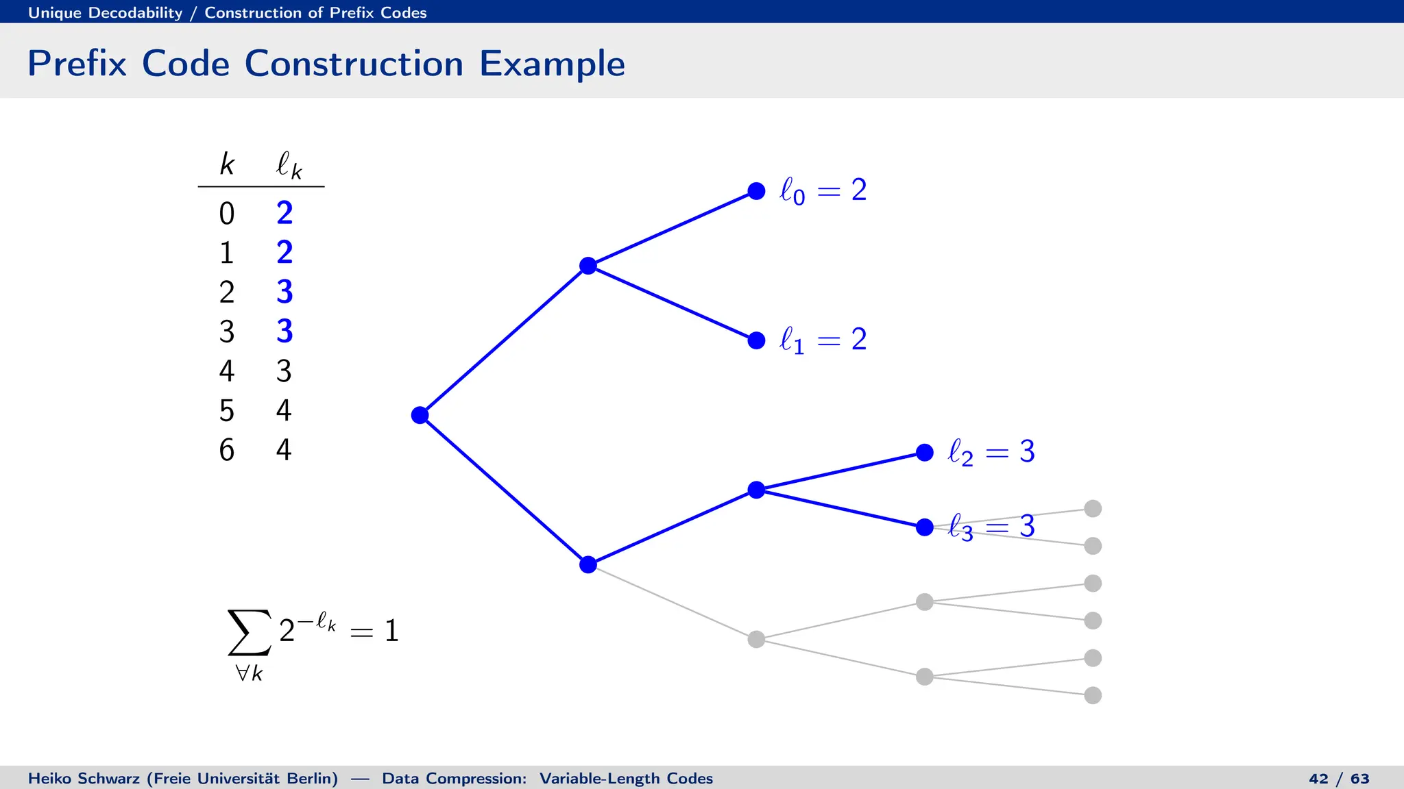
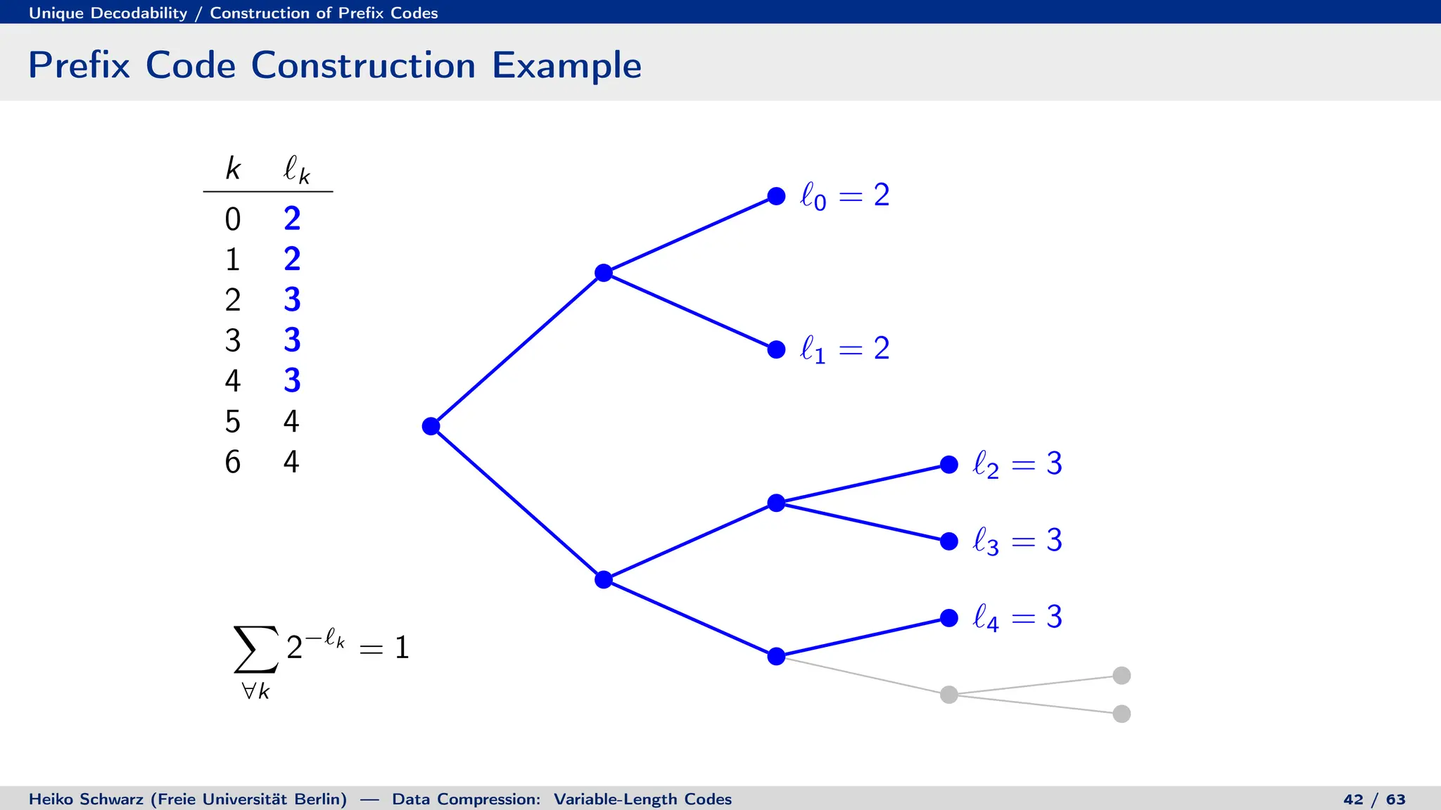
Binary Code Trees for Prefix Codes
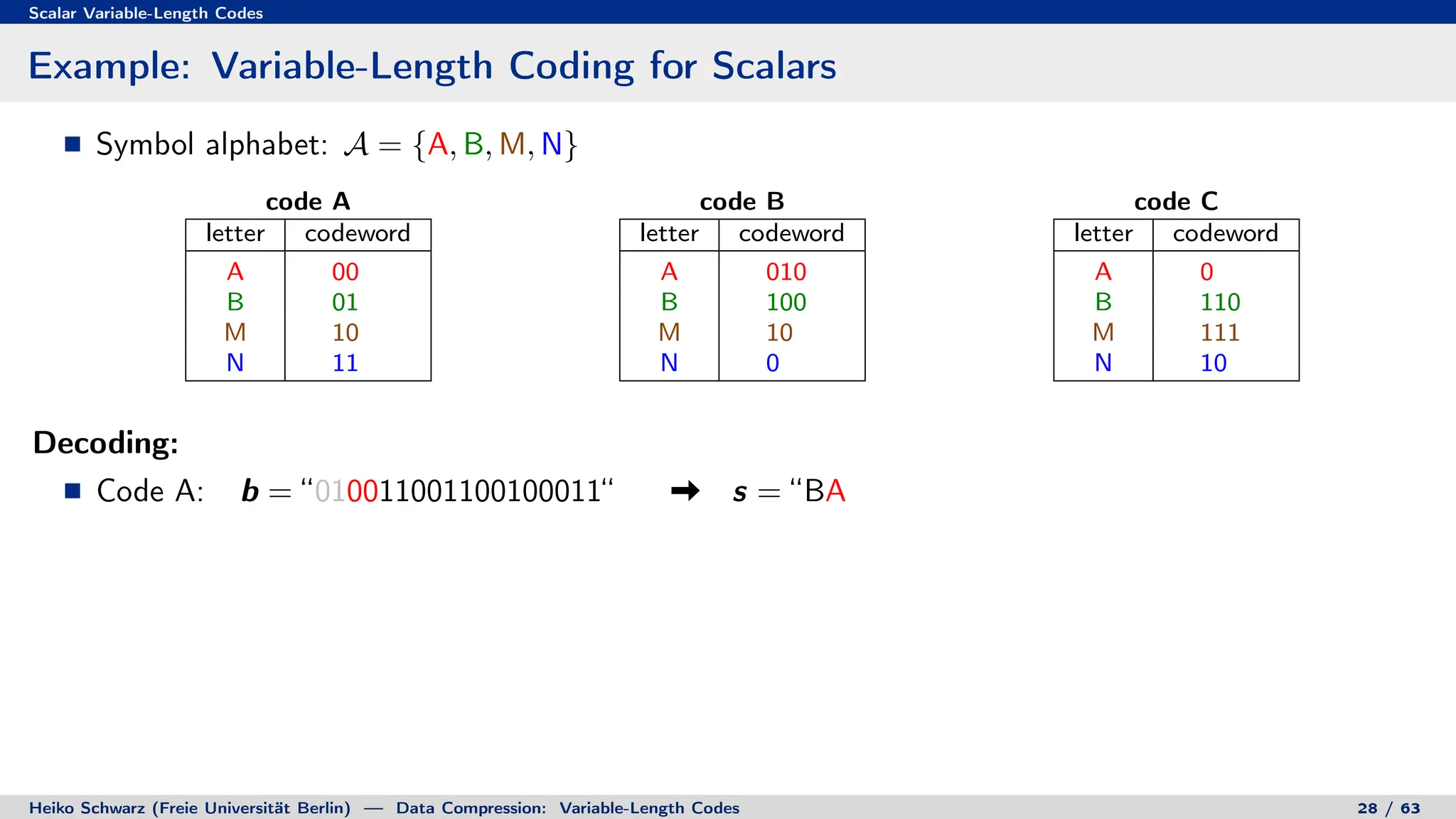
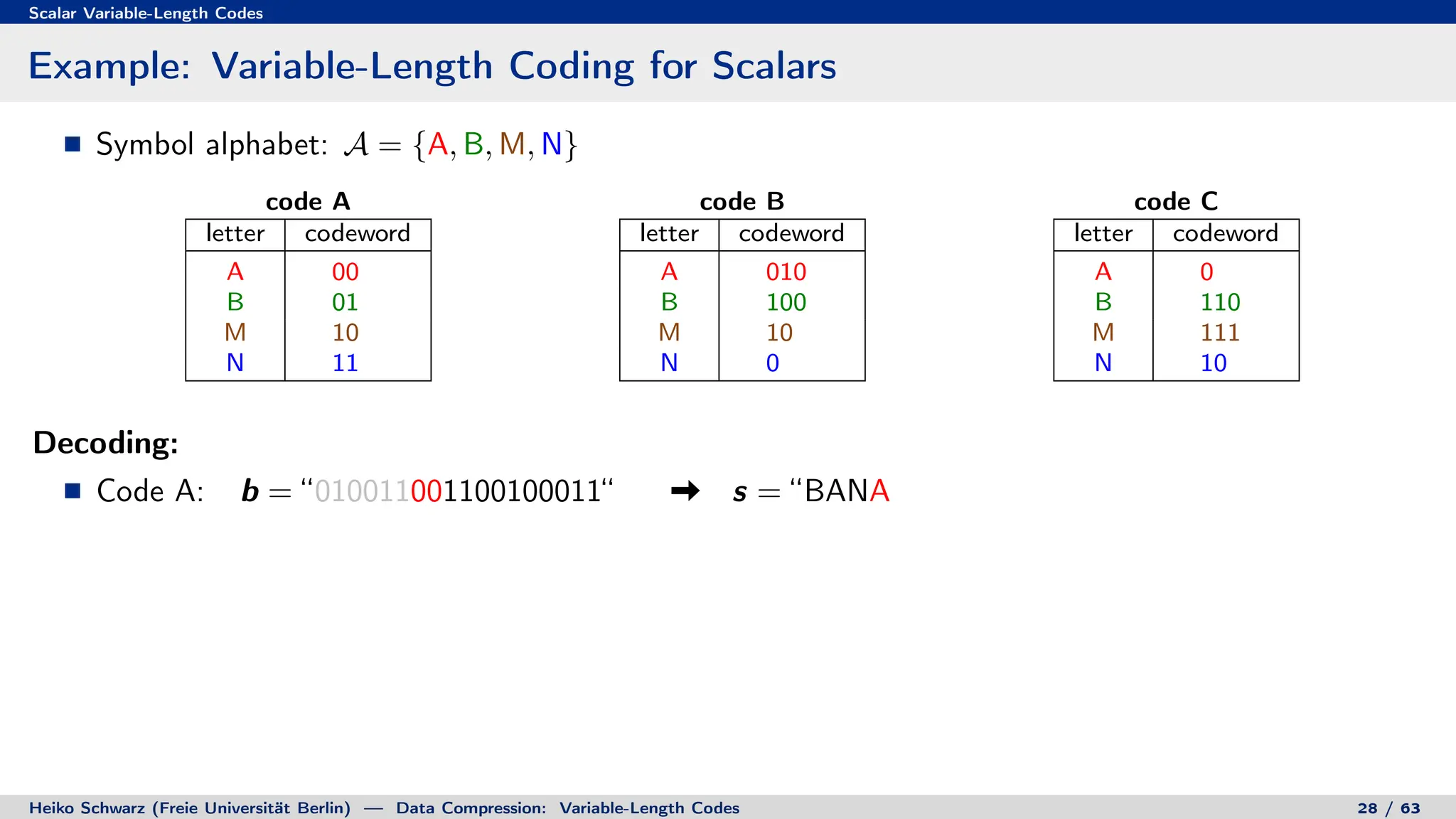
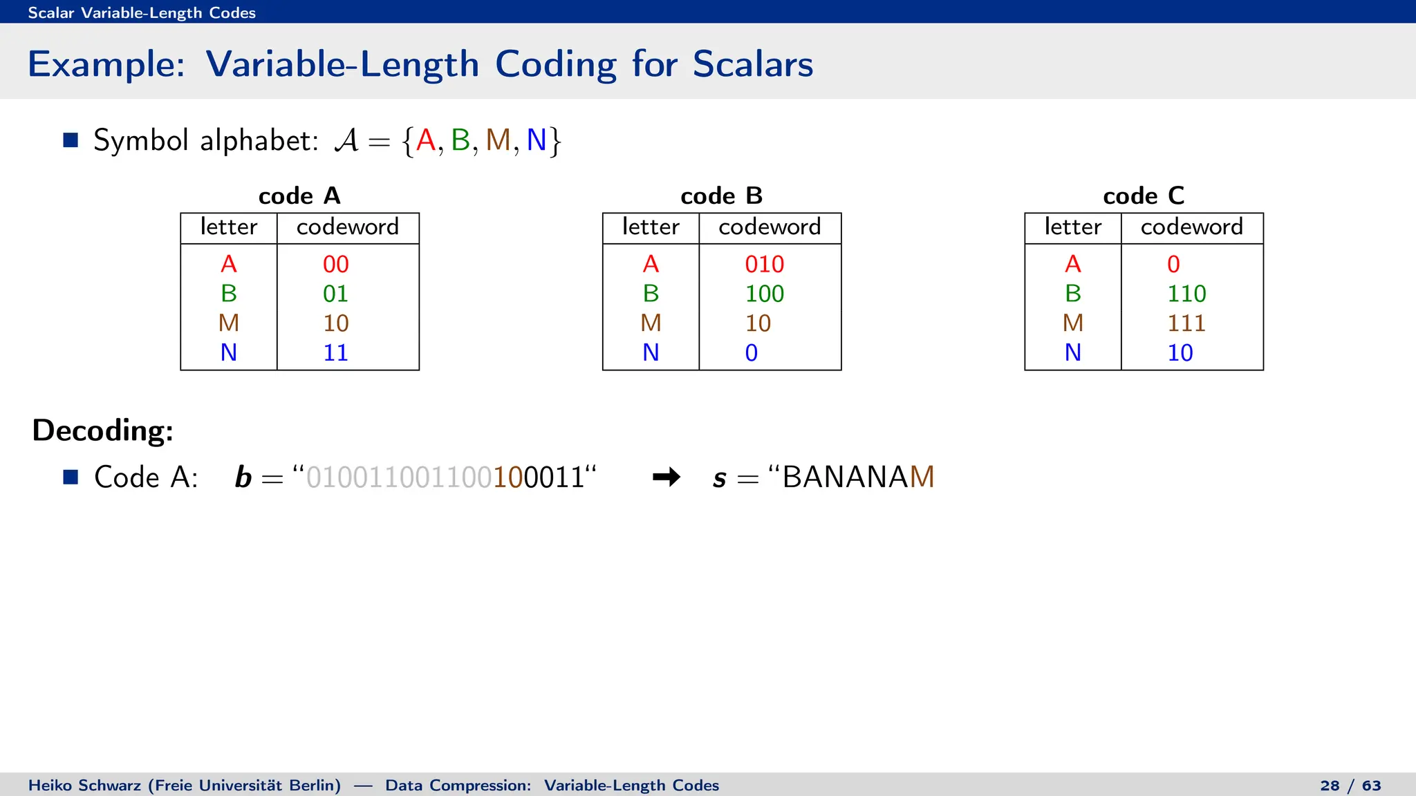
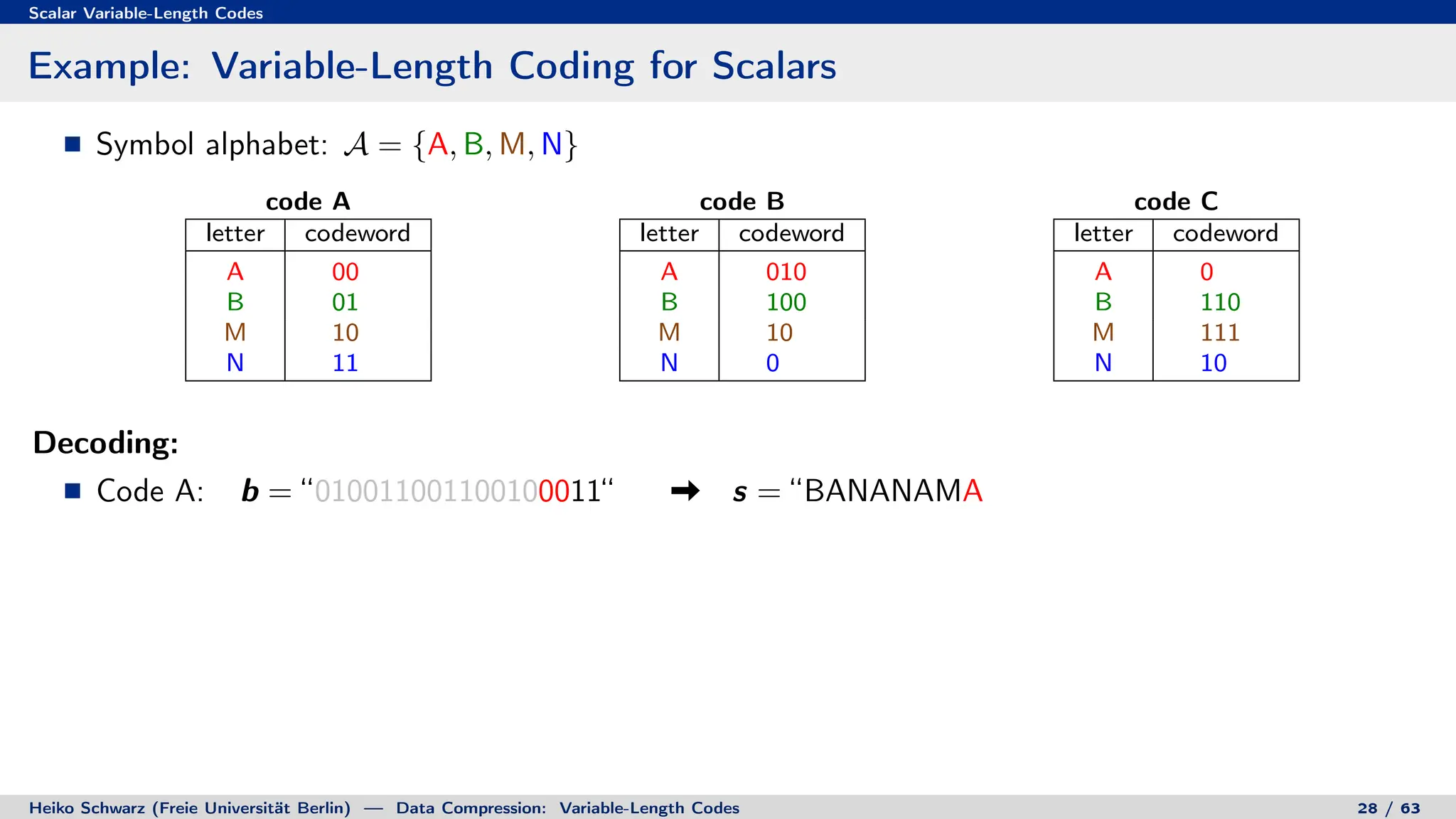
Prefix codes can be represented as binary code trees
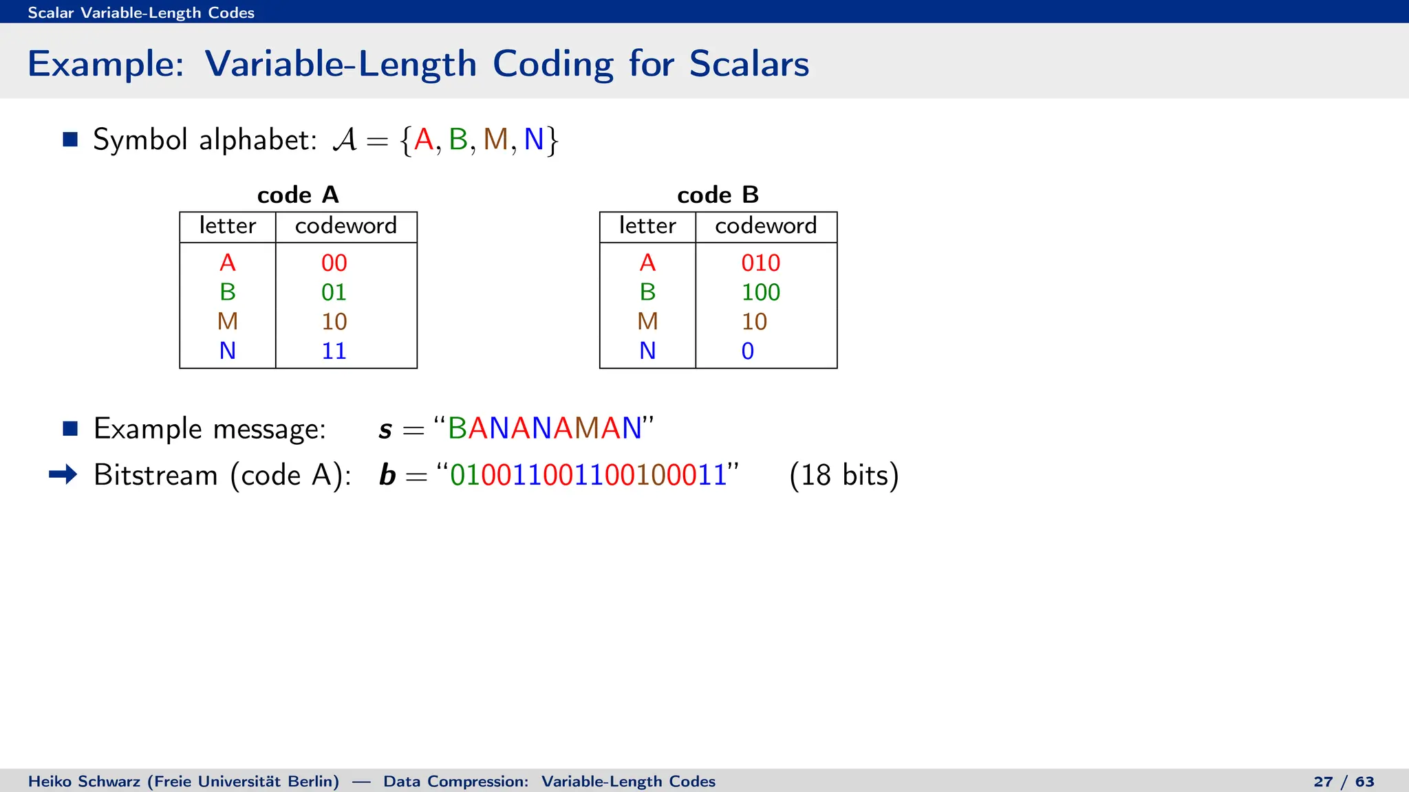
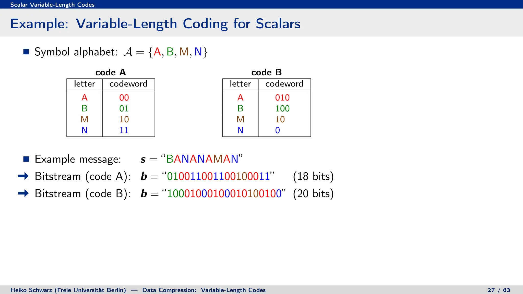
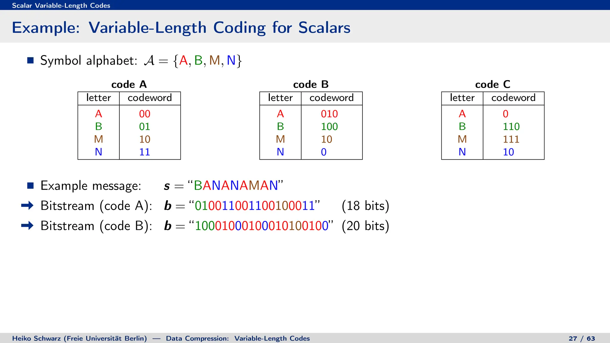
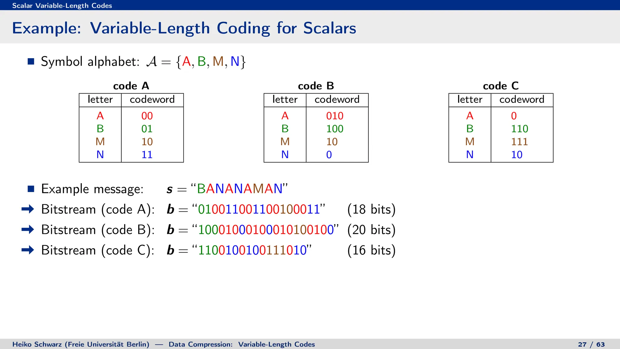
Alphabet letters are assigned to terminal nodes
Codewords are given by labels on path from the root to a terminal node
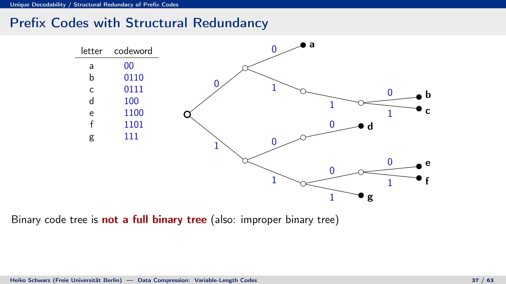
letter codeword
a 00
b 010
c 011
d 10
e 1100
f 1101
g 111
0
0
1
0
1
1 0
1
0
0
1
1
root
node
a [00]
b [010]
c [011]
d [10]
e [1100]
f [1101]
g [111]
Heiko Schwarz (Freie Universität Berlin) — Data Compression: Variable-Length Codes 32 / 63](https://image.slidesharecdn.com/02-variablelengthcodespres-231011080102-7ca4d35b/75/02-VariableLengthCodes_pres-pdf-79-2048.jpg)


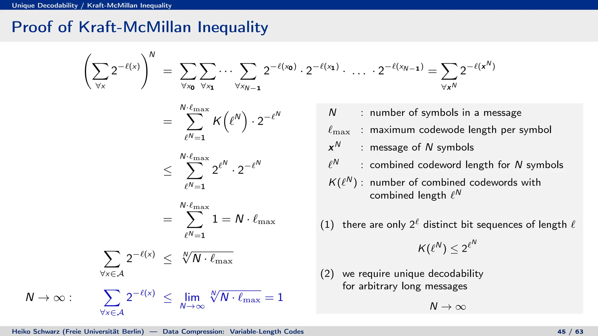


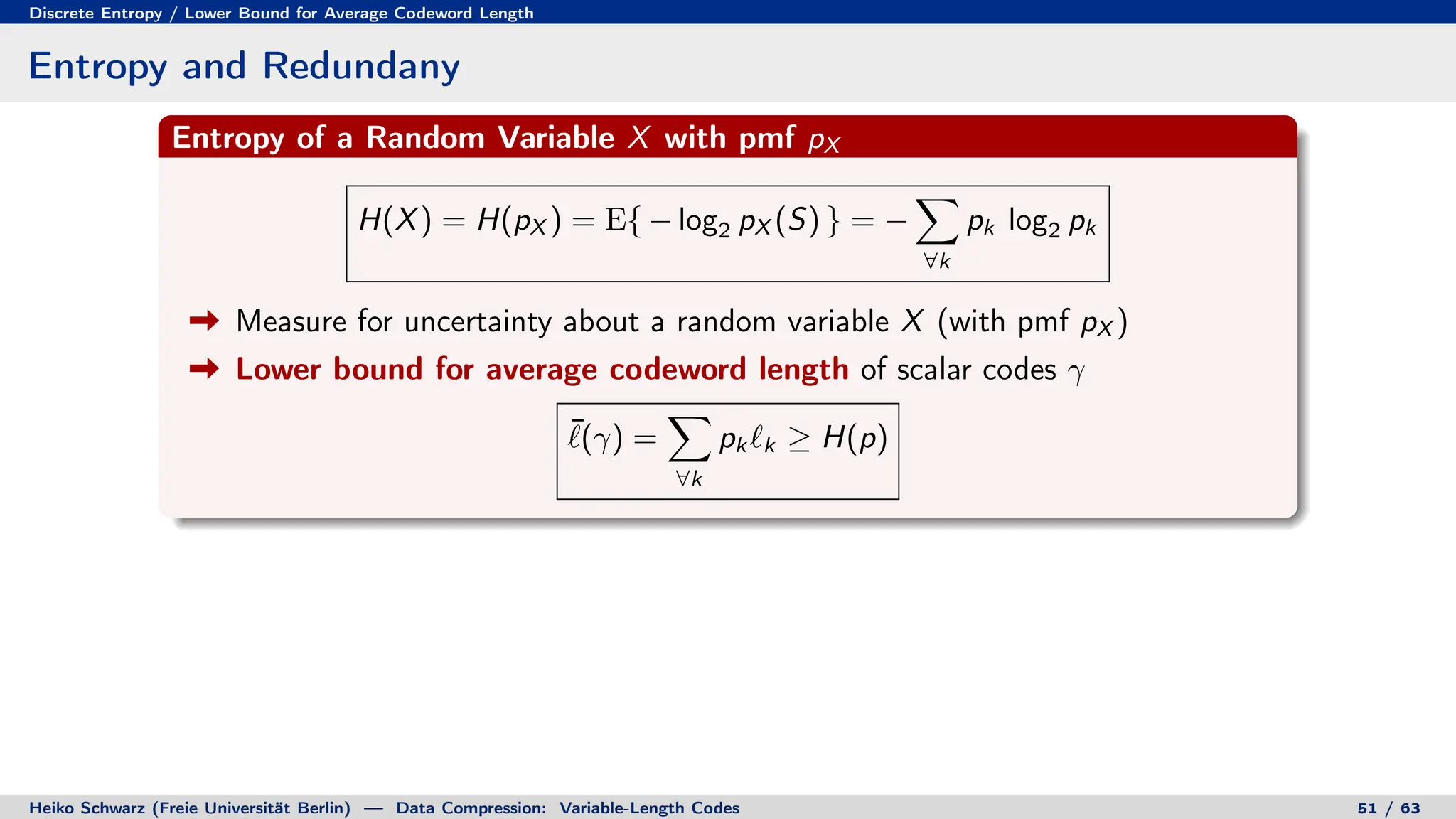
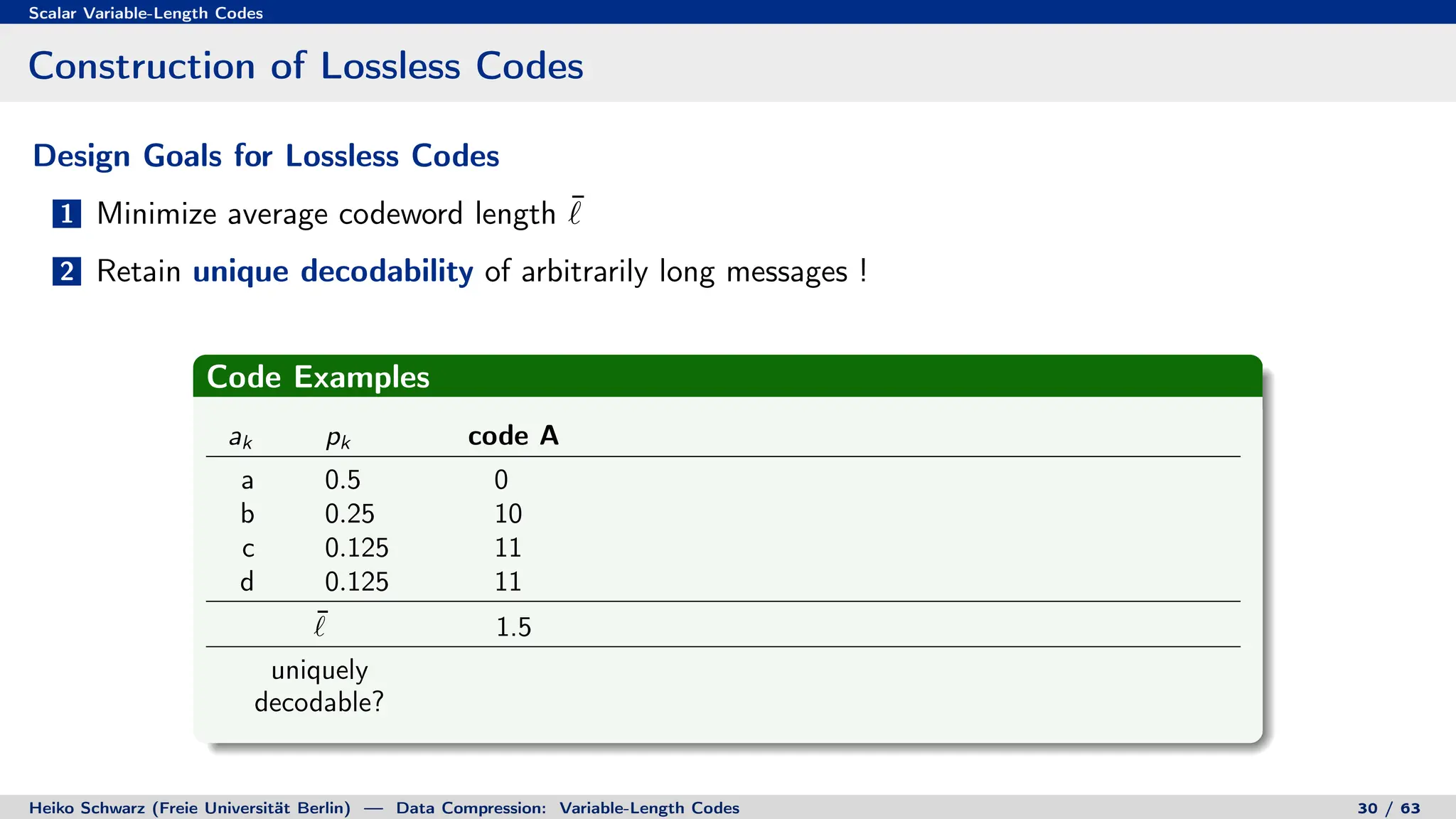
![Discrete Entropy / Lower Bound for Average Codeword Length
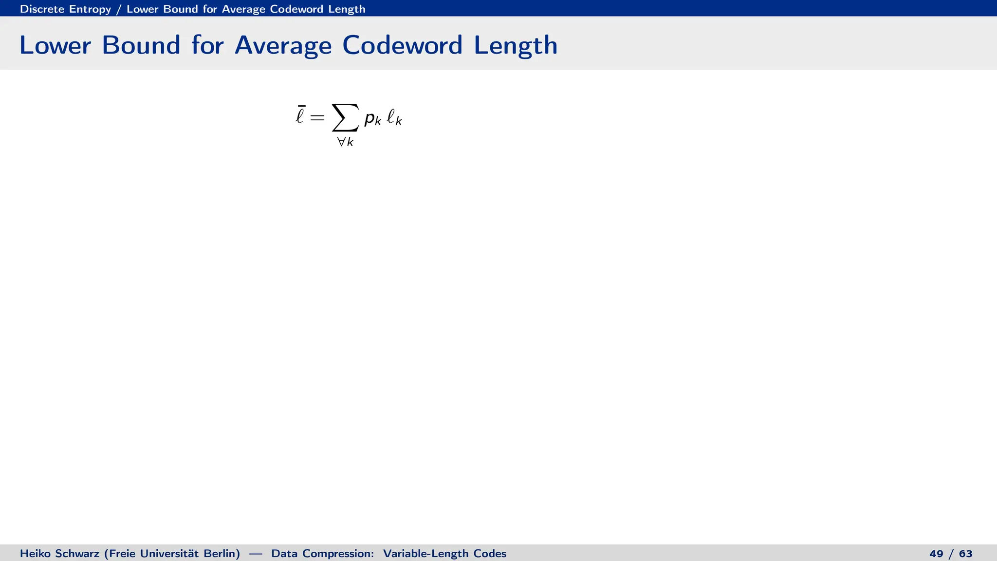
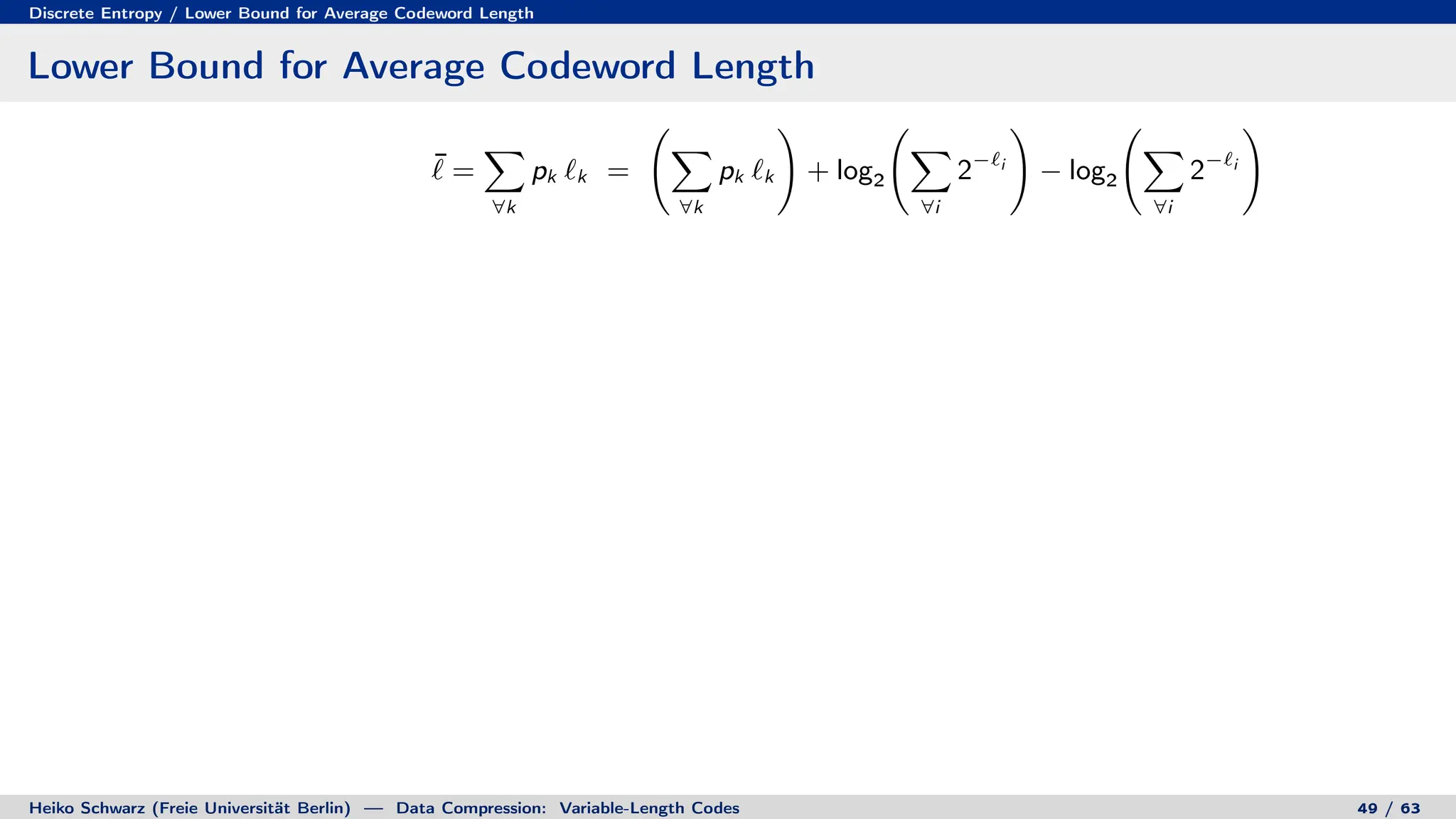
Lower Bound for Average Codeword Length
¯
` =
X
∀k
pk `k =
X
∀k
pk `k
!
+ log2
X
∀i
2−`i
!
− log2
X
∀i
2−`i
!
[ Kraft-McMillan inequality ]
Heiko Schwarz (Freie Universität Berlin) — Data Compression: Variable-Length Codes 49 / 63](https://image.slidesharecdn.com/02-variablelengthcodespres-231011080102-7ca4d35b/75/02-VariableLengthCodes_pres-pdf-153-2048.jpg)
![Discrete Entropy / Lower Bound for Average Codeword Length
Lower Bound for Average Codeword Length
¯
` =
X
∀k
pk `k =
X
∀k
pk `k
!
+ log2
X
∀i
2−`i
!
− log2
X
∀i
2−`i
!
[ Kraft-McMillan inequality ] ≥
X
∀k
pk `k
!
+ log2
X
∀i
2−`i
!
Heiko Schwarz (Freie Universität Berlin) — Data Compression: Variable-Length Codes 49 / 63](https://image.slidesharecdn.com/02-variablelengthcodespres-231011080102-7ca4d35b/75/02-VariableLengthCodes_pres-pdf-154-2048.jpg)
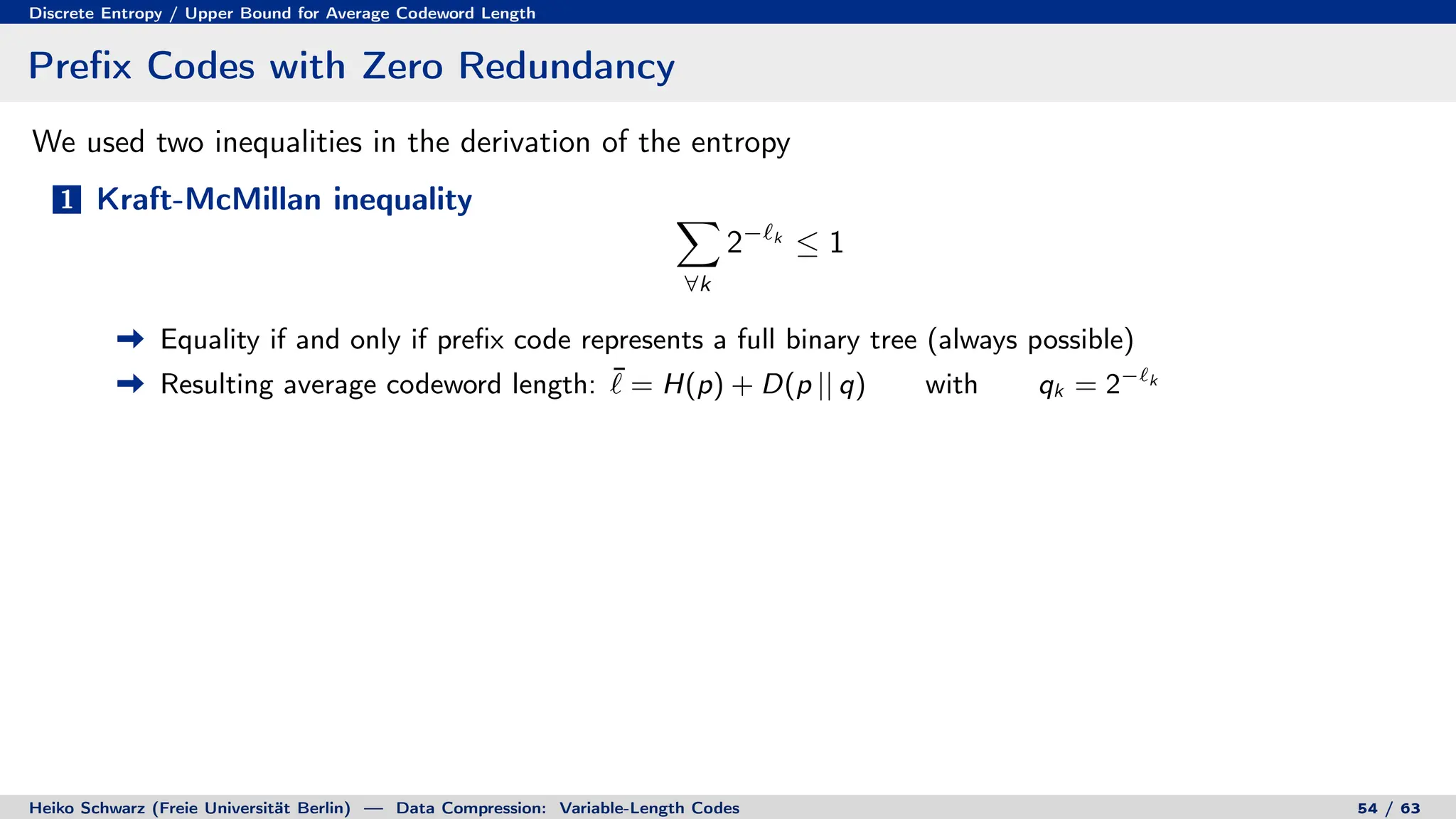
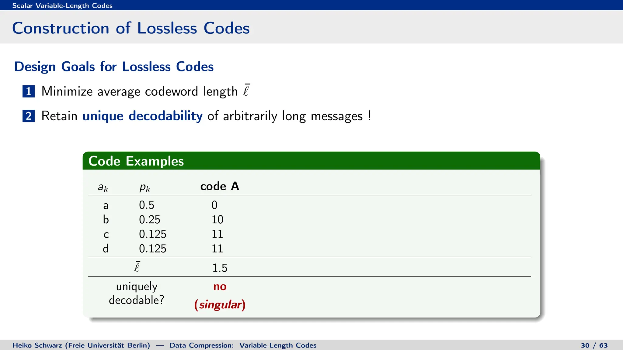
![Discrete Entropy / Lower Bound for Average Codeword Length
Lower Bound for Average Codeword Length
¯
` =
X
∀k
pk `k =
X
∀k
pk `k
!
+ log2
X
∀i
2−`i
!
− log2
X
∀i
2−`i
!
[ Kraft-McMillan inequality ] ≥
X
∀k
pk `k
!
+ log2
X
∀i
2−`i
!
=
X
∀k
pk `k
!
+
X
∀k
pk
!
log2
X
∀i
2−`i
!
Heiko Schwarz (Freie Universität Berlin) — Data Compression: Variable-Length Codes 49 / 63](https://image.slidesharecdn.com/02-variablelengthcodespres-231011080102-7ca4d35b/75/02-VariableLengthCodes_pres-pdf-155-2048.jpg)
![Discrete Entropy / Lower Bound for Average Codeword Length
Lower Bound for Average Codeword Length
¯
` =
X
∀k
pk `k =
X
∀k
pk `k
!
+ log2
X
∀i
2−`i
!
− log2
X
∀i
2−`i
!
[ Kraft-McMillan inequality ] ≥
X
∀k
pk `k
!
+ log2
X
∀i
2−`i
!
=
X
∀k
pk `k
!
+
X
∀k
pk
!
log2
X
∀i
2−`i
!
=
X
∀k
pk `k + log2
X
∀i
2−`i
!!
Heiko Schwarz (Freie Universität Berlin) — Data Compression: Variable-Length Codes 49 / 63](https://image.slidesharecdn.com/02-variablelengthcodespres-231011080102-7ca4d35b/75/02-VariableLengthCodes_pres-pdf-156-2048.jpg)
![Discrete Entropy / Lower Bound for Average Codeword Length
Lower Bound for Average Codeword Length
¯
` =
X
∀k
pk `k =
X
∀k
pk `k
!
+ log2
X
∀i
2−`i
!
− log2
X
∀i
2−`i
!
[ Kraft-McMillan inequality ] ≥
X
∀k
pk `k
!
+ log2
X
∀i
2−`i
!
=
X
∀k
pk `k
!
+
X
∀k
pk
!
log2
X
∀i
2−`i
!
=
X
∀k
pk `k + log2
X
∀i
2−`i
!!
=
X
∀k
pk − log2
2−`k
+ log2
X
∀i
2−`i
!!
Heiko Schwarz (Freie Universität Berlin) — Data Compression: Variable-Length Codes 49 / 63](https://image.slidesharecdn.com/02-variablelengthcodespres-231011080102-7ca4d35b/75/02-VariableLengthCodes_pres-pdf-157-2048.jpg)
![Discrete Entropy / Lower Bound for Average Codeword Length
Lower Bound for Average Codeword Length
¯
` =
X
∀k
pk `k =
X
∀k
pk `k
!
+ log2
X
∀i
2−`i
!
− log2
X
∀i
2−`i
!
[ Kraft-McMillan inequality ] ≥
X
∀k
pk `k
!
+ log2
X
∀i
2−`i
!
=
X
∀k
pk `k
!
+
X
∀k
pk
!
log2
X
∀i
2−`i
!
=
X
∀k
pk `k + log2
X
∀i
2−`i
!!
=
X
∀k
pk − log2
2−`k
+ log2
X
∀i
2−`i
!!
= −
X
∀k
pk log2
2−`k
P
∀i 2−`i
Heiko Schwarz (Freie Universität Berlin) — Data Compression: Variable-Length Codes 49 / 63](https://image.slidesharecdn.com/02-variablelengthcodespres-231011080102-7ca4d35b/75/02-VariableLengthCodes_pres-pdf-158-2048.jpg)
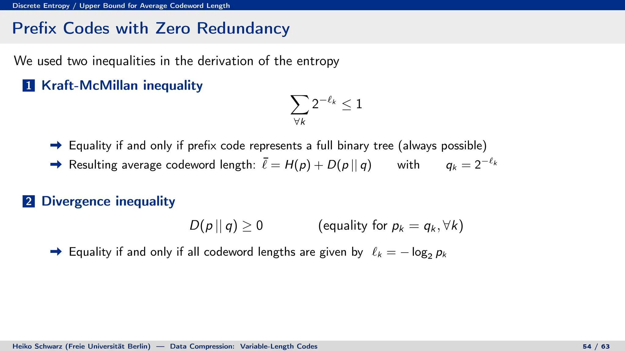
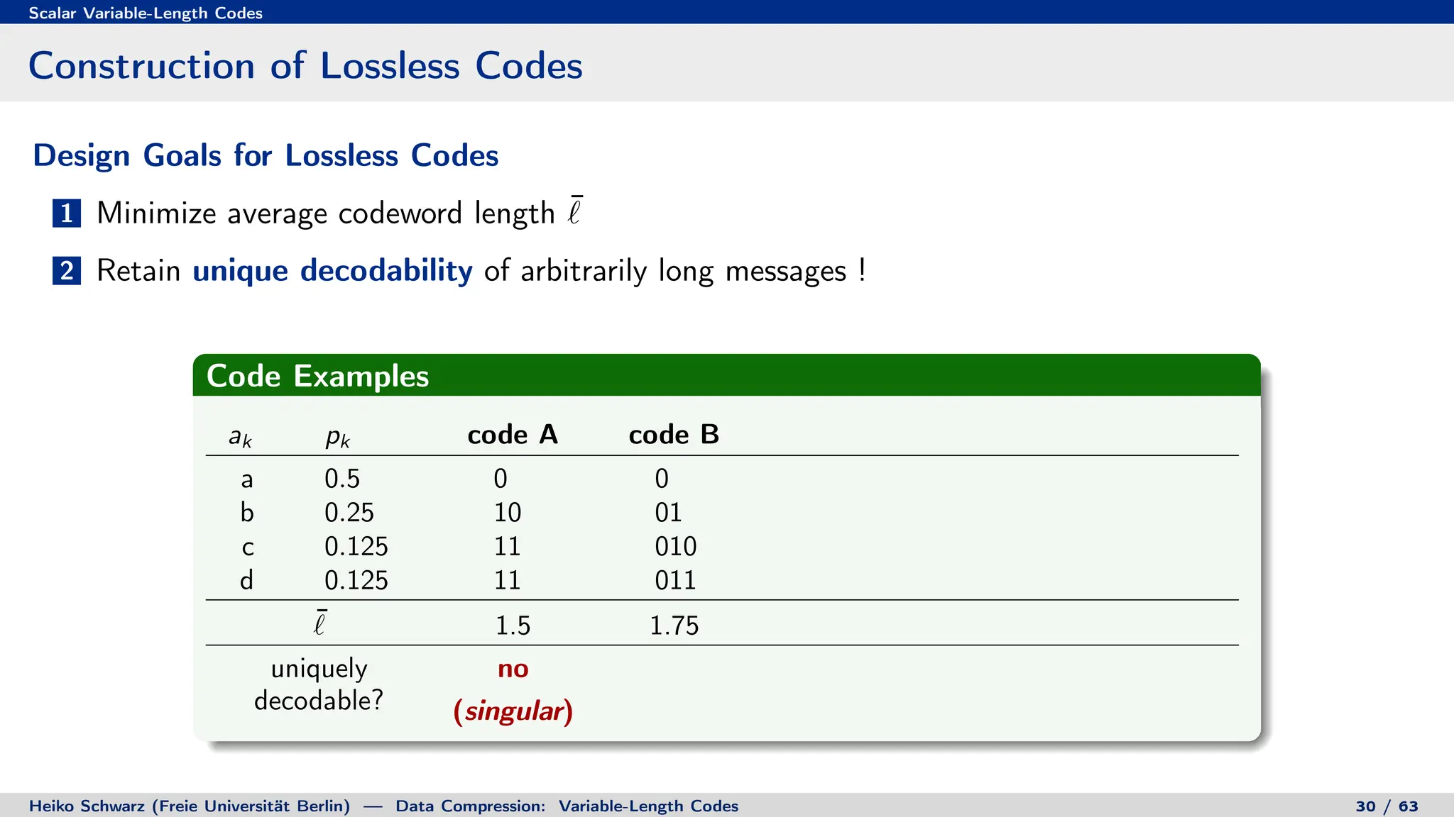
![Discrete Entropy / Lower Bound for Average Codeword Length
Lower Bound for Average Codeword Length (continued)
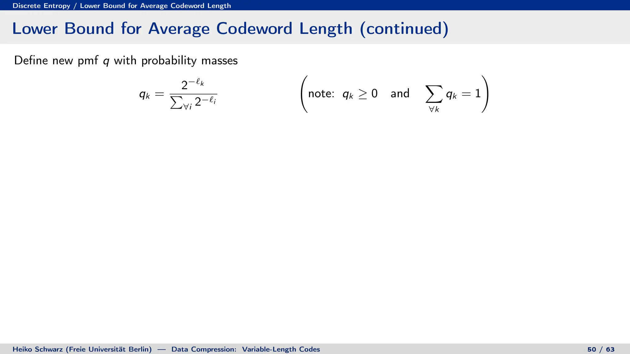
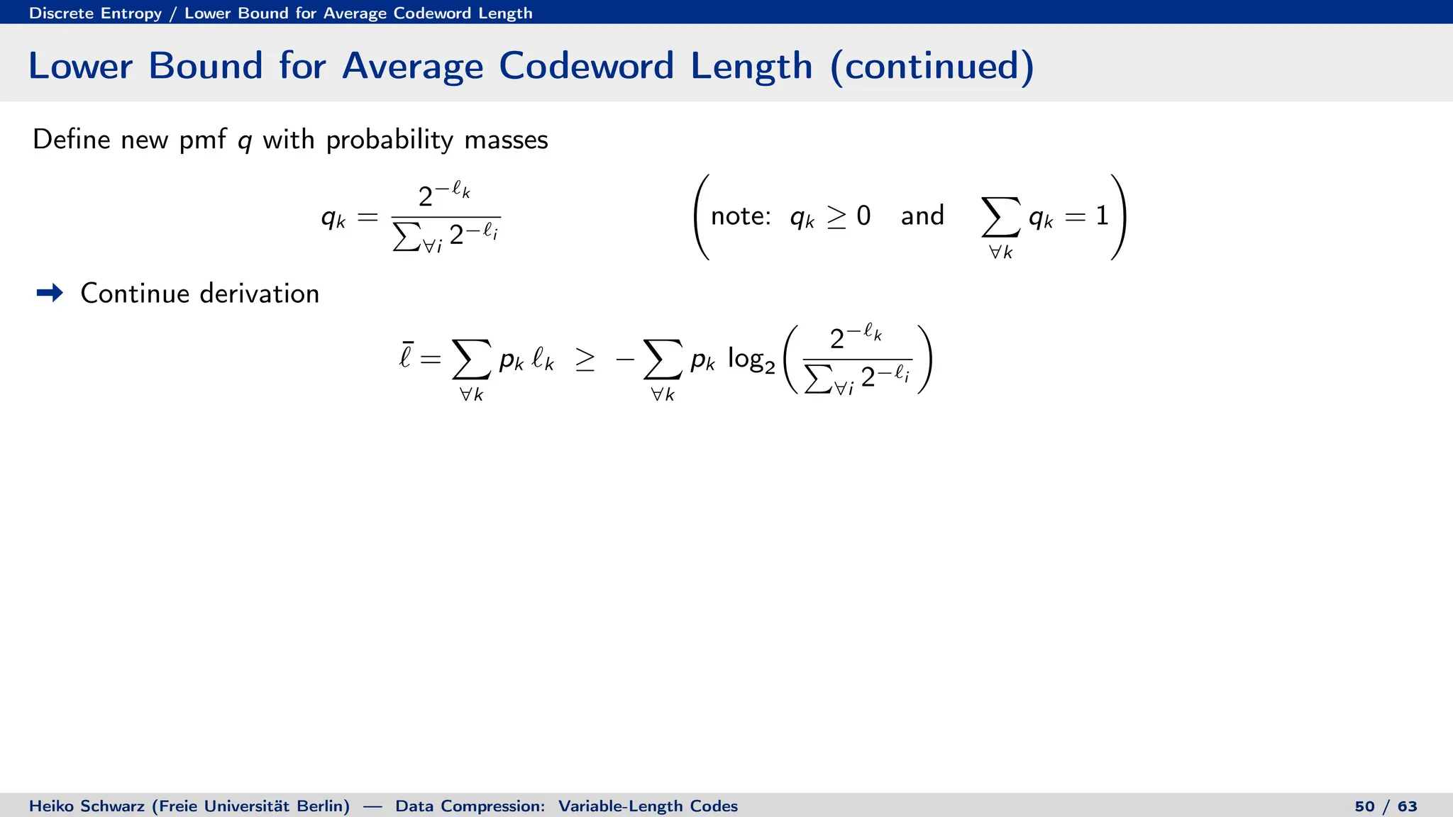
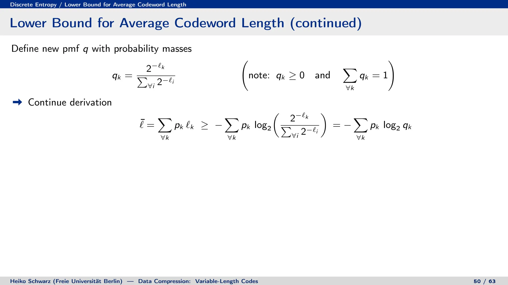
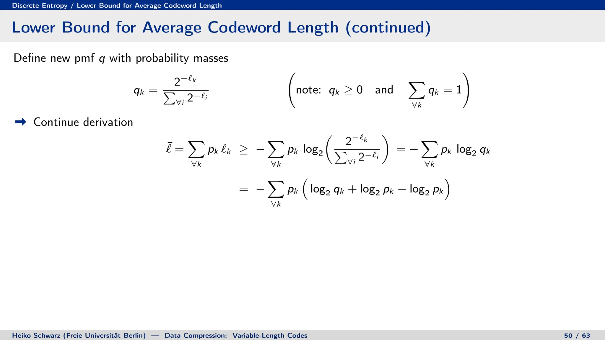
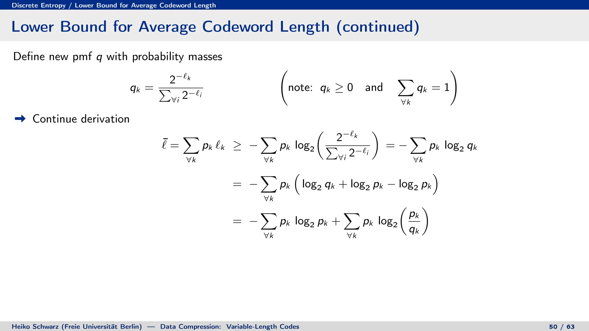
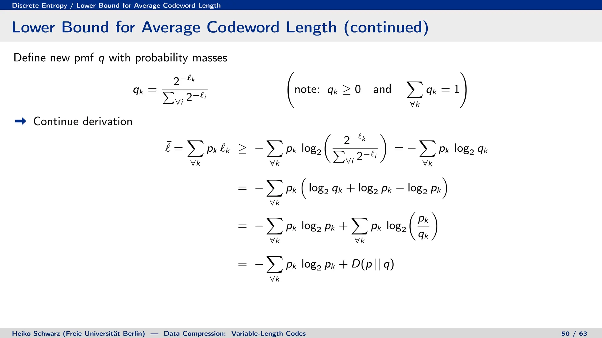
Define new pmf q with probability masses
qk =
2−`k
P
∀i 2−`i
note: qk ≥ 0 and
X
∀k
qk = 1
!
Continue derivation
¯
` =
X
∀k
pk `k ≥ −
X
∀k
pk log2
2−`k
P
∀i 2−`i
= −
X
∀k
pk log2 qk
= −
X
∀k
pk
log2 qk + log2 pk − log2 pk
= −
X
∀k
pk log2 pk +
X
∀k
pk log2
pk
qk
= −
X
∀k
pk log2 pk + D(p || q)
[ divergence inequality ]
Heiko Schwarz (Freie Universität Berlin) — Data Compression: Variable-Length Codes 50 / 63](https://image.slidesharecdn.com/02-variablelengthcodespres-231011080102-7ca4d35b/75/02-VariableLengthCodes_pres-pdf-165-2048.jpg)
![Discrete Entropy / Lower Bound for Average Codeword Length
Lower Bound for Average Codeword Length (continued)
Define new pmf q with probability masses
qk =
2−`k
P
∀i 2−`i
note: qk ≥ 0 and
X
∀k
qk = 1
!
Continue derivation
¯
` =
X
∀k
pk `k ≥ −
X
∀k
pk log2
2−`k
P
∀i 2−`i
= −
X
∀k
pk log2 qk
= −
X
∀k
pk
log2 qk + log2 pk − log2 pk
= −
X
∀k
pk log2 pk +
X
∀k
pk log2
pk
qk
= −
X
∀k
pk log2 pk + D(p || q)
[ divergence inequality ] ≥ −
X
∀k
pk log2 pk
Heiko Schwarz (Freie Universität Berlin) — Data Compression: Variable-Length Codes 50 / 63](https://image.slidesharecdn.com/02-variablelengthcodespres-231011080102-7ca4d35b/75/02-VariableLengthCodes_pres-pdf-166-2048.jpg)