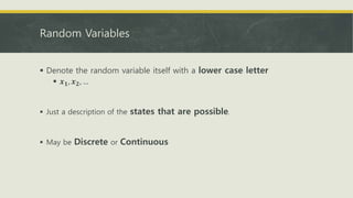
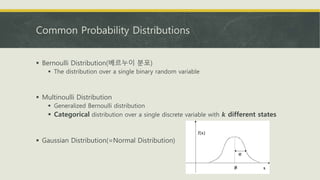
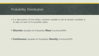
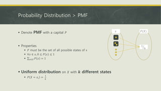
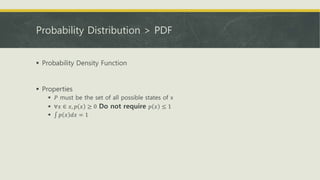
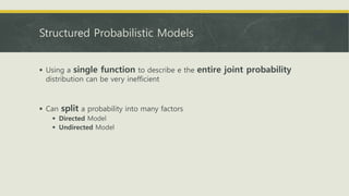
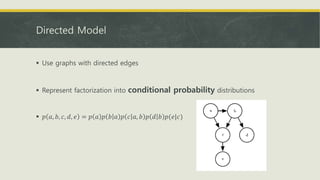
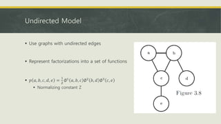
This document discusses key concepts in probability and information theory, including: - Random variables that can take on discrete or continuous states, described by probability mass functions or probability density functions. - Common probability distributions like the Bernoulli, Gaussian, and exponential distributions. - Information theory concepts like entropy, Kullback-Leibler divergence, and how to structure probabilistic models as directed or undirected graphs.

1. Probability &
Information
Theory
2017. 09. 25
Presented by Choi SeongJae

2. Random Variables
 Denote the random variable itself with a lower case letter
 𝒙 𝟏, 𝒙 𝟐, …
 Just a description of the states that are possible.
 May be Discrete or Continuous

3. Probability Distribution
 Is a description of how likely a random variable or set of random variables is
to take on each of its possible states
 Discrete Variables & Probability Mass Functions(PMF)
 Continuous Variables & Probability Density Functions(PDF)

4. Probability Distribution > PMF
 Denote PMF with a capital 𝑃
 Properties
 𝑃 must be the set of all possible states of x
 ∀𝑥 ∈ 𝑥, 0 ≤ 𝑃 𝑥 ≤ 1
 𝑥∈𝑋 𝑃 𝑥 = 1
 Uniform distribution on 𝑋 with 𝒌 different states
 𝑃 𝑋 = 𝑥𝑖 =
1
𝑘
𝑥 𝑃(𝑋)
1
6

5. Probability Distribution > PDF
 Probability Density Function
 Properties
 𝑃 must be the set of all possible states of x
 ∀𝑥 ∈ 𝑥, 𝑝 𝑥 ≥ 0 Do not require 𝑝 𝑥 ≤ 1
 𝑝 𝑥 𝑑𝑥 = 1

6. Marginal Probability(주변확률)
 Joint probability 𝑝(𝑥, 𝑦)만 알 경우, 𝑝(𝑥)의 확률을 구하려고 할 때 사용
 Discrete variable
 ∀𝑥 ∈ 𝑥, 𝑃 𝑋 = 𝑥 = 𝑦 𝑃(𝑋 = 𝑥 𝑌 = 𝑦)
 Continuous variable
 𝑝 𝑥 = 𝑝 𝑥, 𝑦 𝑑𝑦

7. Conditional Probability(조건부 확률)
 𝑌 = 𝑦 given X = 𝑥 as 𝑃(𝑌 = 𝑦|𝑋 = 𝑥)
 𝑃 𝑌 = 𝑦 𝑋 = 𝑥 =
𝑃(𝑌=𝑦,𝑋=𝑥)
𝑃(𝑋=𝑥)

8. Chain Rule of Conditional Probabilities
 Joint probability distribution may be decomposed into conditional
distributions
 𝑷 𝒙 𝟏, 𝒙 𝟐, … , 𝒙 𝒏 = 𝑷(𝒙 𝟏) 𝒊=𝟐
𝒏
𝑷(𝒙𝒊|𝒙 𝟏, … , 𝒙 𝒊−𝟏 )

9. Independence and Conditional Independence
 두 확률의 곱으로 나타낼 수 있으면 𝑥, 𝑦는 Independent
 ∀𝑥 ∈ 𝑥,𝑦 ∈ 𝑦, 𝑝 𝑋 = 𝑥, 𝑌 = 𝑦 = 𝑝 𝑋 = 𝑥 𝑝 𝑌 = 𝑦
 아래 조건을 만족하면 𝑥, 𝑦는 Conditional Independence
 ∀𝑥 ∈ 𝑥, 𝑦 ∈ 𝑦, 𝑧 ∈ 𝑧, 𝑝 𝑋 = 𝑥, 𝑌 = 𝑦 𝑍 = 𝑧 = 𝑝 𝑋 = 𝑥 𝑍 = 𝑧 𝑝 𝑌 = 𝑦 𝑍 = 𝑧
 𝑥 ⊥ 𝑦

10. Expectation(기댓값), Variance(분산) and Covariance(공분산)
 Expectation
 𝔼 𝑥~𝑝 𝑓 𝑥 = 𝑥 𝑃 𝑥 𝑓(𝑥)
 𝔼 𝑥~𝑝 𝑓 𝑥 = 𝑝 𝑥 𝑓 𝑥 𝑑𝑥
 Mean value
 Variance
 𝑉𝑎𝑟 𝑓 𝑥 = 𝔼 (𝑓 𝑥 − 𝔼 𝑓 𝑥 )2
 Covariance
 𝐶𝑜𝑣(𝑓 𝑥 , 𝑔 𝑦 ) = 𝔼 (𝑓 𝑥 − 𝔼 𝑓 𝑥 )(𝑔 𝑦 − 𝔼[𝑔(𝑦)])
 𝑥, 𝑦 사이에 선형관계가 있으면 𝐶𝑜𝑣는 양 또는 음의 값을 갖음
 선형관계가 존재하지 않으면 0
 𝐶𝑜𝑣가 0일지라도 선형관계 외의 관계가 존재할 수 있음

11. Common Probability Distributions
 Bernoulli Distribution(베르누이 분포)
 The distribution over a single binary random variable
 Multinoulli Distribution
 Generalized Bernoulli distribution
 Categorical distribution over a single discrete variable with 𝒌 different states
 Gaussian Distribution(=Normal Distribution)

12. Bernoulli Distribution
 𝑃 𝑥 = 1 = 𝜙
 𝑃 𝑥 = 0 = 1 − 𝜙
 𝑃 𝑋 = 𝑥 = 𝜙 𝑥
(1 − 𝜙)1−𝑥
 𝔼 𝑥 = 𝜙
 𝑉𝑎𝑟 𝑥 = 𝜙 1 − 𝜙
 Binary Entropy
 𝐻 𝑥 = −𝔼(log 𝑝(𝑥))
 𝐻 𝑥 = 𝜙 − 1 log 1 − 𝜙 − 𝜙 log 𝜙

13. Gaussian Distribution(정규분포)
 Normal Distribution
 𝒩 𝑥; 𝜇, 𝜎2 =
1
2𝜋𝜎2 𝑒
−
1
2𝜎2(𝑥−𝜇)
 Normal distribution is a good default choice for two major reasons.
 Many distributions we wish to model are truly close to being normal distributions.
 Central limit theorem
 Normal distribution encodes the maximum amount of uncertainty over the real
numbers
 Similar to real world
• Delving Deep into Rectifiers: Surpassing Human-Level Performance on ImageNet Classification, Kaiming He, ICCV 2015
• Understanding the difficulty of training deep feedforward neural networks, Xavier Glorot, Yoshua Bengio, AISTATS 2010

14. Gaussian Distribution > Central Limit Theorem(중심극한정리)

15. Exponential and Laplace Distributions

16. Mixture of Distribution
 Probability distributions by combining other simpler probability distributions
 𝑃 𝑥 = 𝑖 𝑃 𝑐 = 𝑖 𝑃(𝑥|𝑐 = 𝑖)
 Gaussian Mixture Model(GMM)

17. Useful Function: Logistic Sigmoid
 Commonly used to produce the 𝜙 parameter of a Bernoulli distribution
 𝜎 𝑥 =
1
1+exp(−𝑥)
 Saturates to (0,1)

18. Bayes’ Rule
 𝑃 𝑥 𝑦 =
𝑃 𝑥 𝑃(𝑦|𝑥)
𝑃(𝑦)

19. Information Theory

20. Information Theory
 Mathematics that revolves around quantifying how much information is
present in a signal
 “The sun rose this morning” -> uninformative
 “There was a solar eclipse this morning” -> informative
 Intuitions
 Likely events should have low information content
 Less likely events should have higher information content
 𝐼 𝑥 = − log 𝑃(𝑥)

21. Shannon Entropy
 Can quantify the amount of uncertainty in an entire probability distribution
using the Shannon entropy
 𝐻 𝑥 = 𝔼 𝑥~𝑃 𝐼 𝑥 = −𝔼 𝑥~𝑃[𝑙𝑜𝑔𝑃 𝑥 ]

22. Kullback-Leibler(KL) Divergence
 To measure how different two distributions are
 𝐷 𝐾𝐿(𝑃| 𝑄 = 𝔼 𝑥~𝑃 log
𝑃 𝑥
𝑄 𝑥
= 𝔼 𝑥~𝑃[log 𝑃 𝑥 − log 𝑄(𝑥)]
 Properties
 Non Negative
 KL Divergence is Asymmetric
 𝐷 𝐾𝐿(𝑃||𝑄) ≠ 𝐷 𝐾𝐿(𝑄||𝑃)

23. Structured Probabilistic Models
 Using a single function to describe e the entire joint probability
distribution can be very inefficient
 Can split a probability into many factors
 Directed Model
 Undirected Model

24. Directed Model
 Use graphs with directed edges
 Represent factorization into conditional probability distributions
 𝑝 𝑎, 𝑏, 𝑐, 𝑑, 𝑒 = 𝑝 𝑎 𝑝 𝑏 𝑎 𝑝 𝑐 𝑎, 𝑏 𝑝 𝑑 𝑏 𝑝(𝑒|𝑐)

25. Undirected Model
 Use graphs with undirected edges
 Represent factorizations into a set of functions
 𝑝 𝑎, 𝑏, 𝑐, 𝑑, 𝑒 =
1
𝑍
∅1 𝑎, 𝑏, 𝑐 ∅2 𝑏, 𝑑 ∅3 𝑐, 𝑒
 Normalizing constant Z