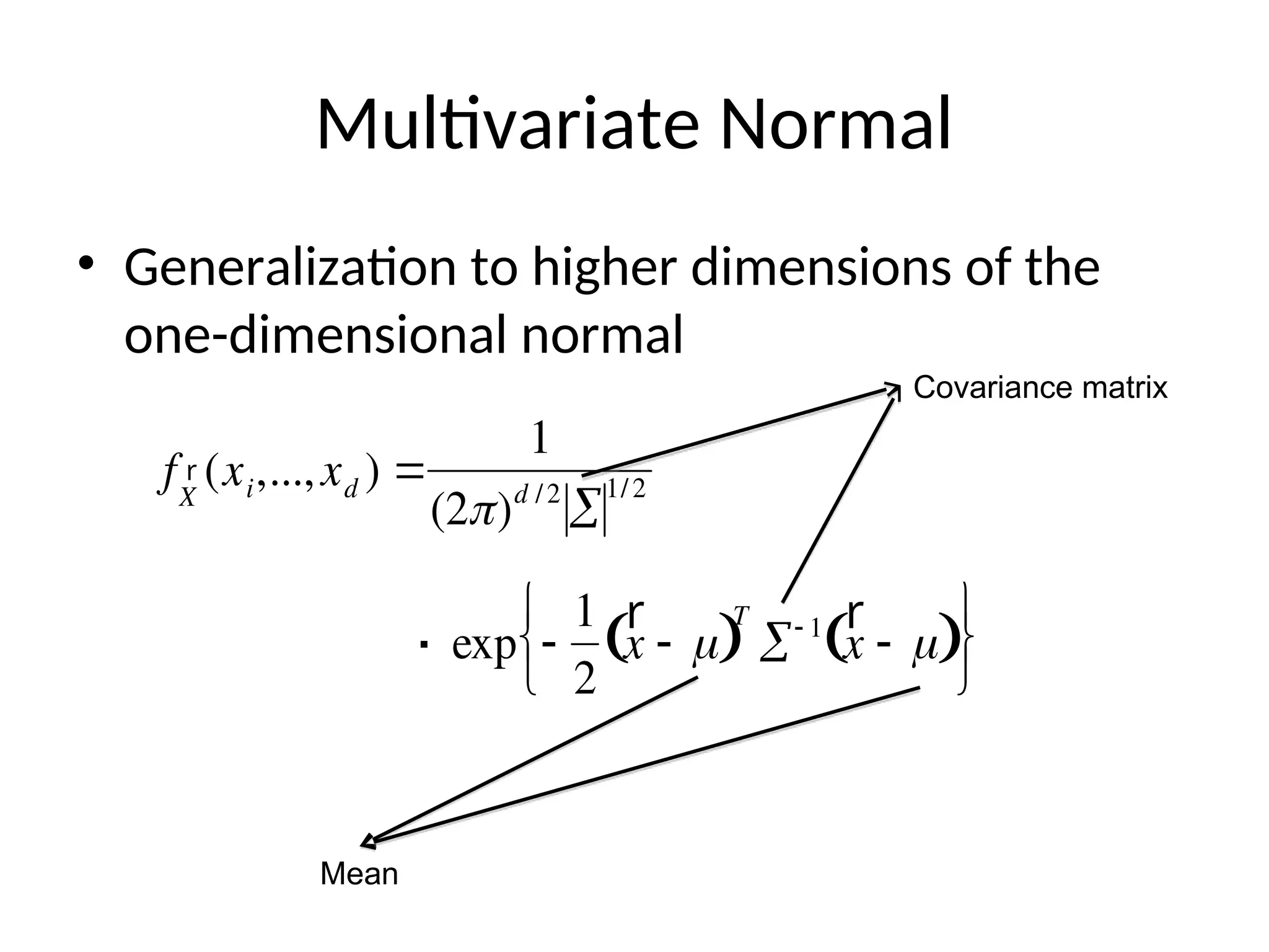
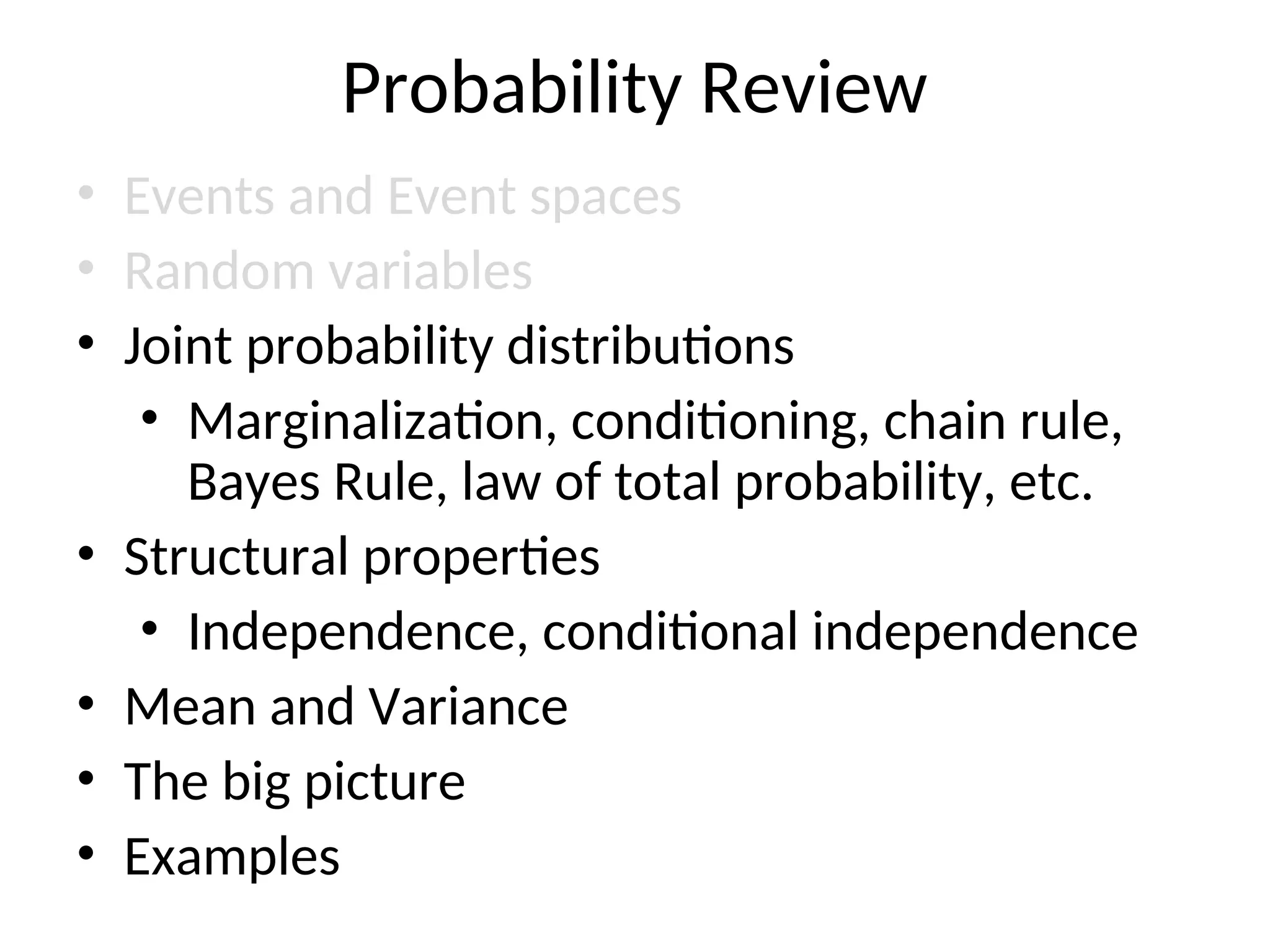
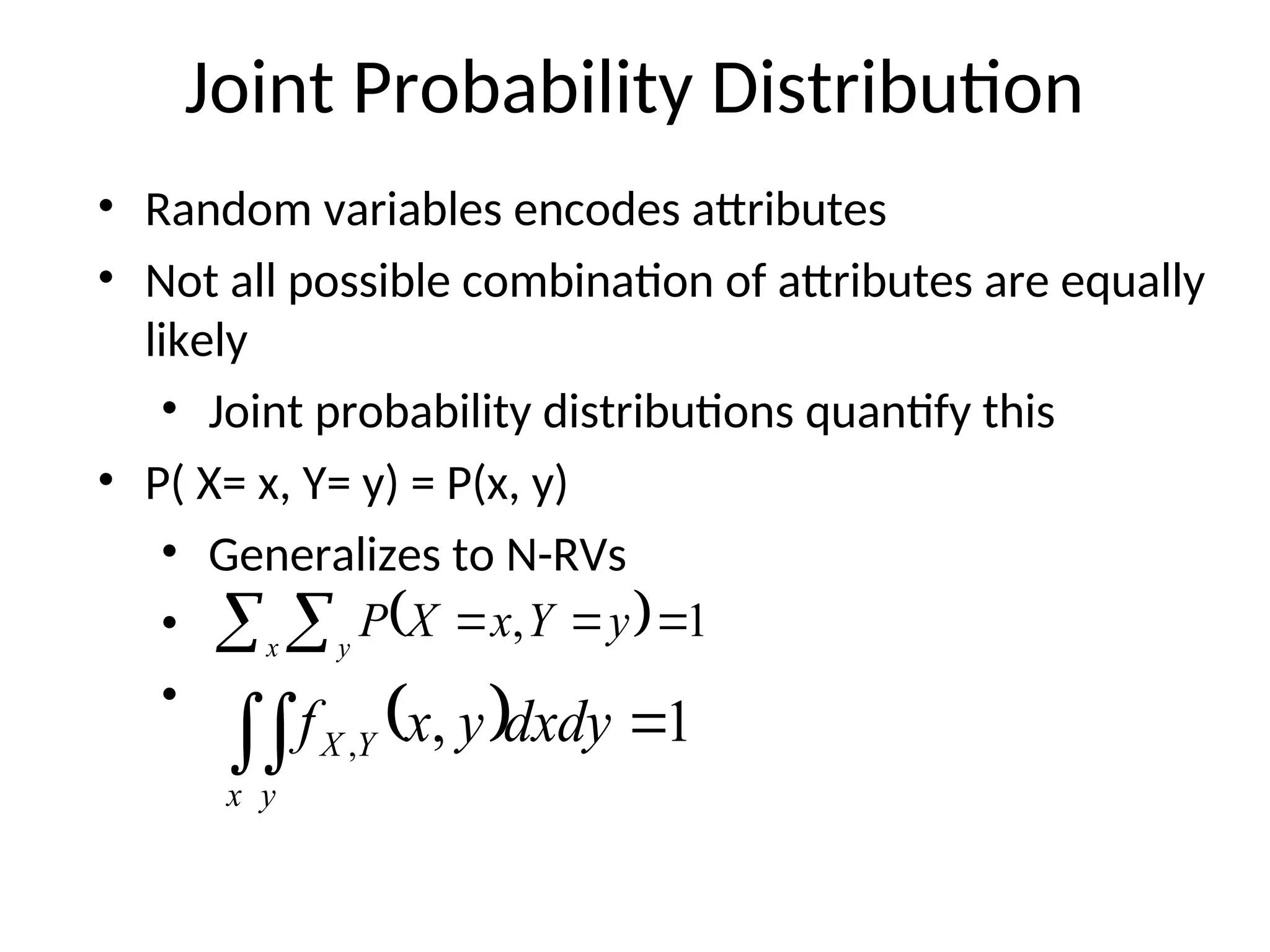
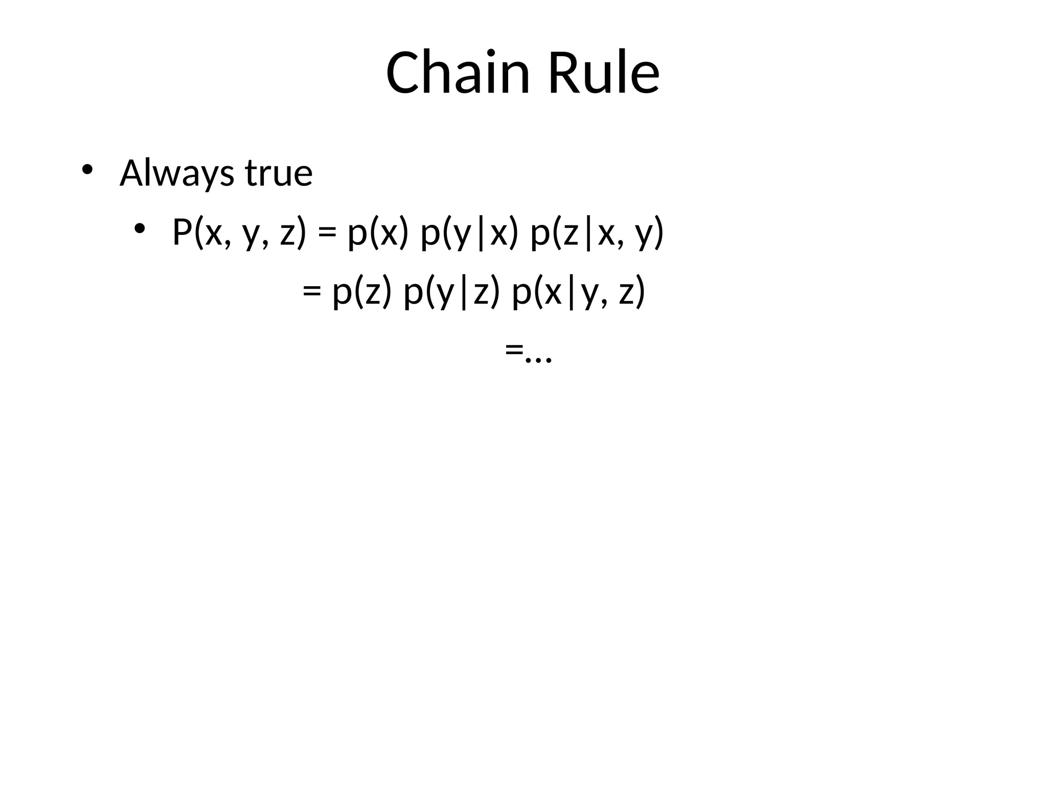
Introduction Lesson in Probability and Review

Probability Review
Thursday Sep 13

Probability Review
• Events and Event spaces
• Random variables
• Joint probability distributions
• Marginalization, conditioning, chain rule,
Bayes Rule, law of total probability, etc.
• Structural properties
• Independence, conditional independence
• Mean and Variance
• The big picture
• Examples

Sample space and Events
• Sample Space, result of an experiment
• If you toss a coin twice 
• Event: a subset of 
• First toss is head = {HH,HT}
• S: event space, a set of events
• Closed under finite union and complements
• Entails other binary operation: union, diff, etc.
• Contains the empty event and 

Probability Measure
• Defined over (Ss.t.
• P() >= 0 for all  in S
• P() = 1
• If  are disjoint, then
• P( U ) = p() + p()
• We can deduce other axioms from the above ones
• Ex: P( U ) for non-disjoint event
P( U ) = p() + p() – p(∩ 

Visualization
• We can go on and define conditional
probability, using the above visualization

Conditional Probability
P(F|H) = Fraction of worlds in which H is true that also
have F true
)
(
)
(
)
|
(
H
p
H
F
p
h
f
p



Rule of total probability
A
B1
B2
B3
B4
B5
B6
B7
     

 i
i B
A
P
B
P
A
p |

From Events to Random Variable
• Almost all the semester we will be dealing with RV
• Concise way of specifying attributes of outcomes
• Modeling students (Grade and Intelligence):
• all possible students
• What are events
• Grade_A = all students with grade A
• Grade_B = all students with grade B
• Intelligence_High = … with high intelligence
• Very cumbersome
• We need “functions” that maps from to an
attribute space.
• P(G = A) = P({student ϵ G(student) = A})

Random Variables

High
low
A
B A+
I:Intelligence
G:Grade
P(I = high) = P( {all students whose intelligence is high})

Discrete Random Variables
• Random variables (RVs) which may take on
only a countable number of distinct values
– E.g. the total number of tails X you get if you flip
100 coins
• X is a RV with arity k if it can take on exactly
one value out of {x1, …, xk}
– E.g. the possible values that X can take on are 0, 1,
2, …, 100

Probability of Discrete RV
• Probability mass function (pmf): P(X = xi)
• Easy facts about pmf
 Σi P(X = xi) = 1
 P(X = xi∩X = xj) = 0 if i ≠ j
 P(X = xi U X = xj) = P(X = xi) + P(X = xj) if i ≠ j
 P(X = x1 U X = x2 U … U X = xk) = 1

Common Distributions
• Uniform X U[1, …, N]
 X takes values 1, 2, … N
 P(X = i) = 1/N
 E.g. picking balls of different colors from a box
• Binomial X Bin(n, p)
 X takes values 0, 1, …, n

 E.g. coin flips

p(X i) 
n
i






pi
(1 p)n i

Continuous Random Variables
• Probability density function (pdf) instead of
probability mass function (pmf)
• A pdf is any function f(x) that describes the
probability density in terms of the input
variable x.

Probability of Continuous RV
• Properties of pdf


• Actual probability can be obtained by taking
the integral of pdf
 E.g. the probability of X being between 0 and 1 is

f (x) 0,x
f (x) 1



P(0 X 1)  f (x)dx
0
1


Cumulative Distribution Function
• FX(v) = P(X ≤ v)
• Discrete RVs
 FX(v) = Σvi P(X = vi)
• Continuous RVs


FX (v)  f (x)dx

v

d
dx
Fx (x)  f (x)

Common Distributions
• Normal X N(μ, σ2
)

 E.g. the height of the entire population

f (x) 
1
 2
exp 
(x  )2
22







Multivariate Normal
• Generalization to higher dimensions of the
one-dimensional normal


f r
X
(xi,...,xd ) 
1
(2)d /2

1/2


exp 
1
2
r
x  
 
T
 1 r
x  
 






.
Covariance matrix
Mean

Joint Probability Distribution
• Random variables encodes attributes
• Not all possible combination of attributes are equally
likely
• Joint probability distributions quantify this
• P( X= x, Y= y) = P(x, y)
• Generalizes to N-RVs
•
•
 
  


x y
y
Y
x
X
P 1
,
 
 
x y
Y
X dxdy
y
x
f 1
,
,

Chain Rule
• Always true
• P(x, y, z) = p(x) p(y|x) p(z|x, y)
= p(z) p(y|z) p(x|y, z)
=…

Conditional Probability
 
 
 
P X Y
P X Y
P Y
x y
x y
y
  
  

 
)
(
)
,
(
|
y
p
y
x
p
y
x
P 
But we will always write it this way:
events

Marginalization
• We know p(X, Y), what is P(X=x)?
• We can use the low of total probability, why?
   
   




y
y
y
x
P
y
P
y
x
P
x
p
|
,
A
B1
B2
B3
B4
B5
B6
B7

Marginalization Cont.
• Another example
   
   




y
z
z
y
z
y
x
P
z
y
P
z
y
x
P
x
p
,
,
,
|
,
,
,

Bayes Rule
• We know that P(rain) = 0.5
• If we also know that the grass is wet, then
how this affects our belief about whether it
rains or not?

P rain | wet
 
P(rain)P(wet | rain)
P(wet)
P x | y
 
P(x)P(y | x)
P(y)

Bayes Rule cont.
• You can condition on more variables
 
)
|
(
)
,
|
(
)
|
(
,
|
z
y
P
z
x
y
P
z
x
P
z
y
x
P 

Independence
• X is independent of Y means that knowing Y
does not change our belief about X.
• P(X|Y=y) = P(X)
• P(X=x, Y=y) = P(X=x) P(Y=y)
• The above should hold for all x, y
• It is symmetric and written as X  Y

Independence
• X1, …, Xn are independent if and only if
• If X1, …, Xn are independent and identically
distributed we say they are iid (or that they
are a random sample) and we write

P(X1  A1,...,Xn  An )  P Xi  Ai
 
i
1
n

X1, …, Xn ∼ P

CI: Conditional Independence
• RV are rarely independent but we can still
leverage local structural properties like
Conditional Independence.
• X  Y | Z if once Z is observed, knowing the
value of Y does not change our belief about X
• P(rain  sprinkler’s on | cloudy)
• P(rain  sprinkler’s on | wet grass)

Mean and Variance
• Mean (Expectation):
– Discrete RVs:
– Continuous RVs:
 
X
E
 
   
X P X
i
i i
v
E v v
 

   
X
E xf x dx

 


E(g(X))  g(vi)P(X vi)
vi

E(g(X))  g(x) f (x)dx




Mean and Variance
• Variance:
– Discrete RVs:
– Continuous RVs:
• Covariance:
• Covariance:
     
2
X P X
i
i i
v
V v v

  

     
2
X
V x f x dx


 
 


Var(X) E((X  )2
)
Var(X) E(X2
)  2
Cov(X,Y) E((X  x )(Y  y )) E(XY)  xy

Mean and Variance
• Correlation:

(X,Y) Cov(X,Y)/xy

 1(X,Y) 1

Properties
• Mean
–
–
– If X and Y are independent,
• Variance
–
– If X and Y are independent,
     
X Y X Y
E E E
  
   
X X
E a aE

     
XY X Y
E E E
 
   
2
X X
V a b a V
 
 
X Y (X) (Y)
V V V
  

Some more properties
• The conditional expectation of Y given X when
the value of X = x is:
• The Law of Total Expectation or Law of
Iterated Expectation:
  dy
x
y
p
y
x
X
Y
E )
|
(
*
| 


   

 dx
x
p
x
X
Y
E
X
Y
E
E
Y
E X )
(
)
|
(
)
|
(
)
(

Some more properties
• The law of Total Variance:

Var(Y) Var E(Y | X)
  E Var(Y | X)
 

The Big Picture
Model Data
Probability
Estimation/learning

Statistical Inference
• Given observations from a model
– What (conditional) independence assumptions
hold?
• Structure learning
– If you know the family of the model (ex,
multinomial), What are the value of the
parameters: MLE, Bayesian estimation.
• Parameter learning

Monty Hall Problem
• You're given the choice of three doors: Behind one
door is a car; behind the others, goats.
• You pick a door, say No. 1
• The host, who knows what's behind the doors, opens
another door, say No. 3, which has a goat.
• Do you want to pick door No. 2 instead?

Host must
reveal Goat B
Host must
reveal Goat A
Host reveals
Goat A
or
Host reveals
Goat B

Monty Hall Problem: Bayes Rule
• : the car is behind door i, i = 1, 2, 3
•
• : the host opens door j after you pick door i
•
i
C
ij
H
  1 3
i
P C 
 
0
0
1 2
1 ,
ij k
i j
j k
P H C
i k
i k j k


 




  


Monty Hall Problem: Bayes Rule cont.
• WLOG, i=1, j=3
•
•
 
   
 
13 1 1
1 13
13
P H C P C
P C H
P H

   
13 1 1
1 1 1
2 3 6
P H C P C   

•
•
       
       
13 13 1 13 2 13 3
13 1 1 13 2 2
, , ,
1 1
1
6 3
1
2
P H P H C P H C P H C
P H C P C P H C P C
  
 
  

 
1 13
1 6 1
1 2 3
P C H  

 
1 13
1 6 1
1 2 3
P C H  


 You should switch!
   
2 13 1 13
1 2
1
3 3
P C H P C H
   

Information Theory
• P(X) encodes our uncertainty about X
• Some variables are more uncertain that others
• How can we quantify this intuition?
• Entropy: average number of bits required to encode X
P(X) P(Y)
X Y
 
 
 
 
 

 









x
x
P x
P
x
P
x
P
x
P
x
p
E
X
H )
(
log
1
log
1
log

Information Theory cont.
• Entropy: average number of bits required to encode X
• We can define conditional entropy similarly
• i.e. once Y is known, we only need H(X,Y) – H(Y) bits
• We can also define chain rule for entropies (not surprising)
 
 
   
Y
H
Y
X
H
y
x
p
E
Y
X
H P
P
P








 ,
|
1
log
|
       
Y
X
Z
H
X
Y
H
X
H
Z
Y
X
H P
P
P
P ,
|
|
,
, 


 
 
 
 
 

 









x
x
P x
P
x
P
x
P
x
P
x
p
E
X
H )
(
log
1
log
1
log

Mutual Information: MI
• Remember independence?
• If XY then knowing Y won’t change our belief about X
• Mutual information can help quantify this! (not the only
way though)
• MI:
• “The amount of uncertainty in X which is removed by
knowing Y”
• Symmetric
• I(X;Y) = 0 iff, X and Y are independent!
     
Y
X
H
X
H
Y
X
I P
P
P |
; 

 








y x y
p
x
p
y
x
p
y
x
p
Y
X
I
)
(
)
(
)
,
(
log
)
,
(
)
;
(

Chi Square Test for Independence
(Example)
Republican Democrat Independent Total
Male 200 150 50 400
Female 250 300 50 600
Total 450 450 100 1000
• State the hypotheses
H0
: Gender and voting preferences are independent.
Ha
: Gender and voting preferences are not independent
• Choose significance level
Say, 0.05

• Analyze sample data
• Degrees of freedom =
|g|-1 * |v|-1 = (2-1) * (3-1) = 2
• Expected frequency count =
Eg,v = (ng * nv) / n
Em,r = (400 * 450) / 1000 = 180000/1000 = 180
Em,d= (400 * 450) / 1000 = 180000/1000 = 180
Em,i = (400 * 100) / 1000 = 40000/1000 = 40
Ef,r = (600 * 450) / 1000 = 270000/1000 = 270
Ef,d = (600 * 450) / 1000 = 270000/1000 = 270
Ef,i = (600 * 100) / 1000 = 60000/1000 = 60
Male 200 150 50 400
Female 250 300 50 600
Total 450 450 100 1000

• Chi-square test statistic
• Χ2
= (200 - 180)2
/180 + (150 - 180)2
/180 + (50 - 40)2
/40 +
(250 - 270)2
/270 + (300 - 270)2
/270 + (50 - 60)2
/40
• Χ2
= 400/180 + 900/180 + 100/40 + 400/270 + 900/270 +
100/60
• Χ2
= 2.22 + 5.00 + 2.50 + 1.48 + 3.33 + 1.67 = 16.2







 
 
v
g
v
g
v
g
E
E
O
X
,
2
,
,
2
)
(
Male 200 150 50 400
Female 250 300 50 600
Total 450 450 100 1000

• P-value
– Probability of observing a sample statistic as
extreme as the test statistic
– P(X2
≥ 16.2) = 0.0003
• Since P-value (0.0003) is less than the
significance level (0.05), we cannot accept the
null hypothesis
• There is a relationship between gender and
voting preference

Acknowledgment
• Carlos Guestrin recitation slides:
http://www.cs.cmu.edu/~guestrin/Class/10708/recitations/r1/Probability_and_St
atistics_Review.ppt
• Andrew Moore Tutorial:
http://www.autonlab.org/tutorials/prob.html
• Monty hall problem:
http://en.wikipedia.org/wiki/Monty_Hall_problem
• http://www.cs.cmu.edu/~guestrin/Class/10701-F07/recitation_schedule.html
• Chi-square test for independence
http://stattrek.com/chi-square-test/independence.aspx

Introduction Lesson in Probability and Review

More Related Content

Similar to Introduction Lesson in Probability and Review

More from Keith Adrian Villaran

Recently uploaded

Introduction Lesson in Probability and Review