Download to read offline
![Common Distributions
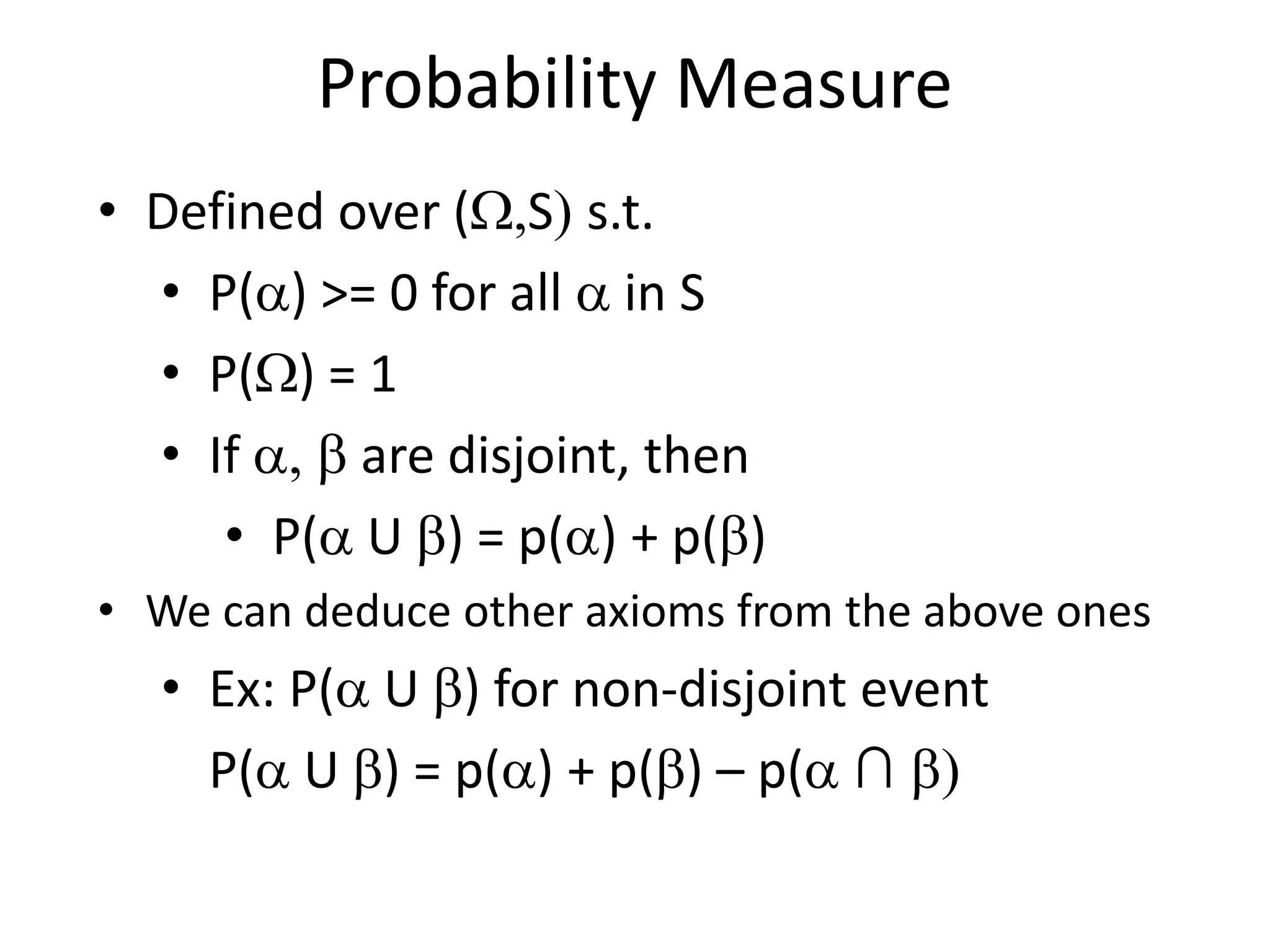
• Uniform X U[1, …, N]
X takes values 1, 2, … N
P(X = i) = 1/N
E.g. picking balls of different colors from a box
• Binomial X Bin(n, p)
X takes values 0, 1, …, n
E.g. coin flips
p(X = i) =
n
i
pi
(1 p)ni](https://image.slidesharecdn.com/probabilityreview-240731042749-8c670d39/75/Probability-Review-for-beginner-to-be-used-for-12-2048.jpg)
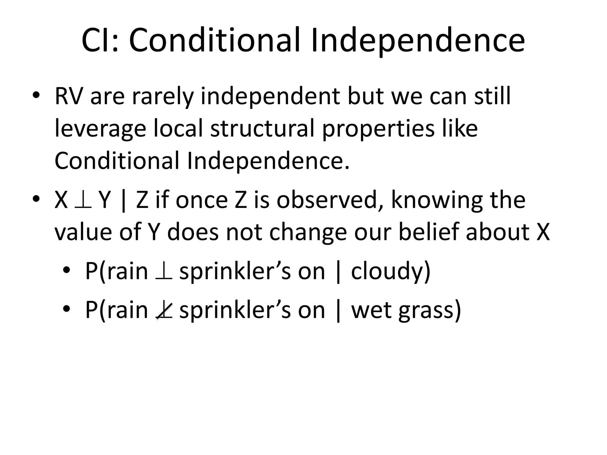
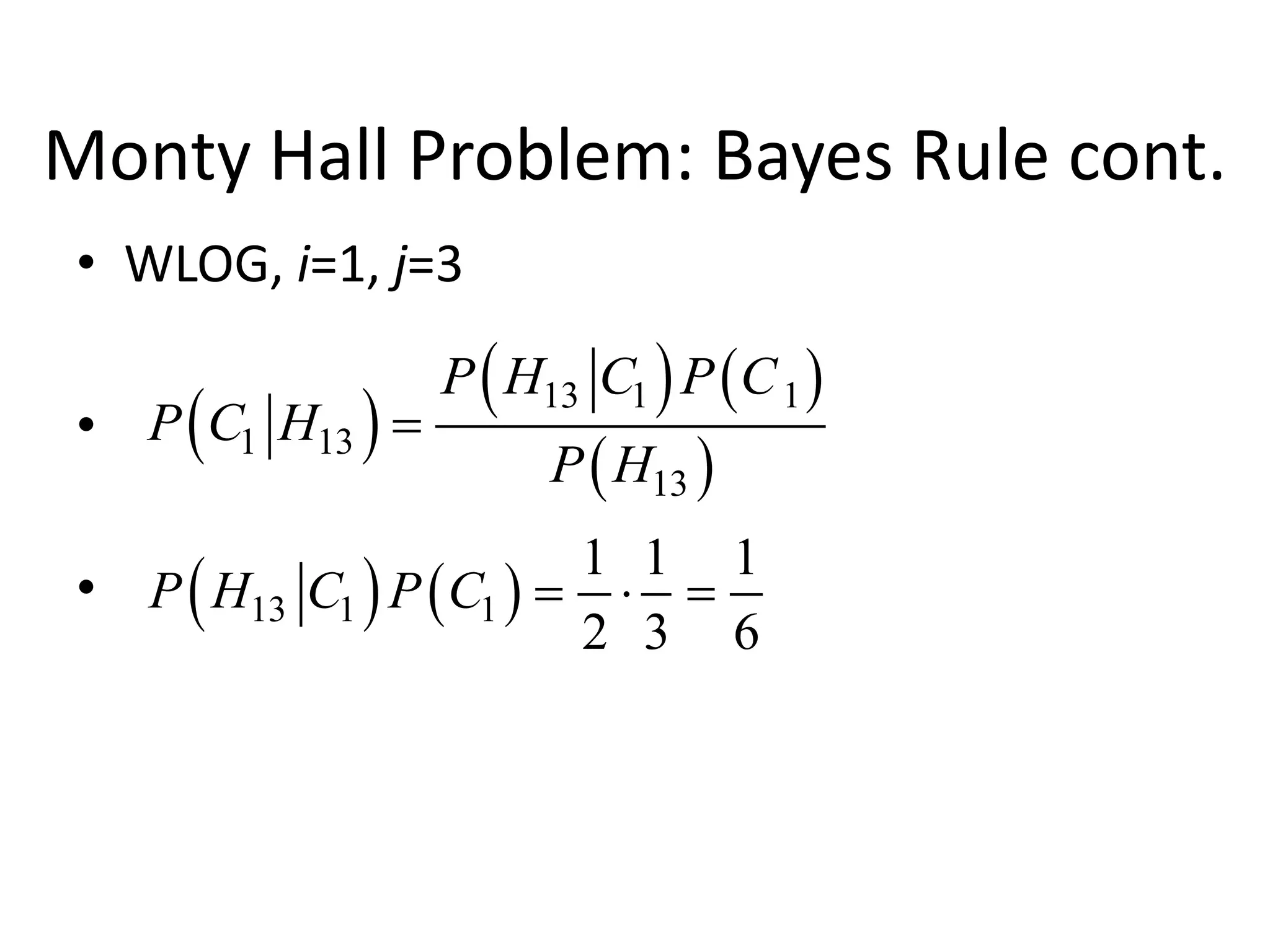
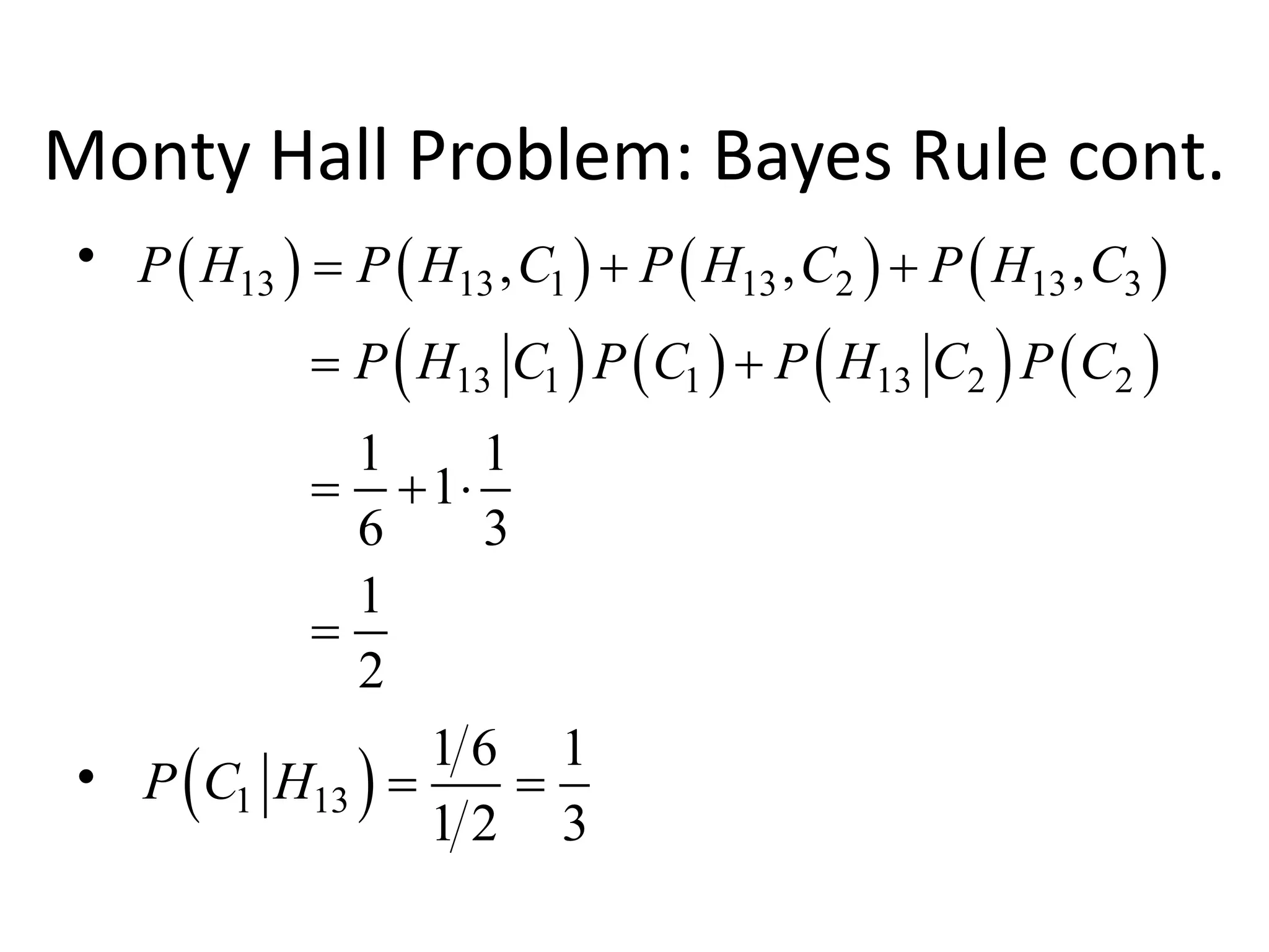
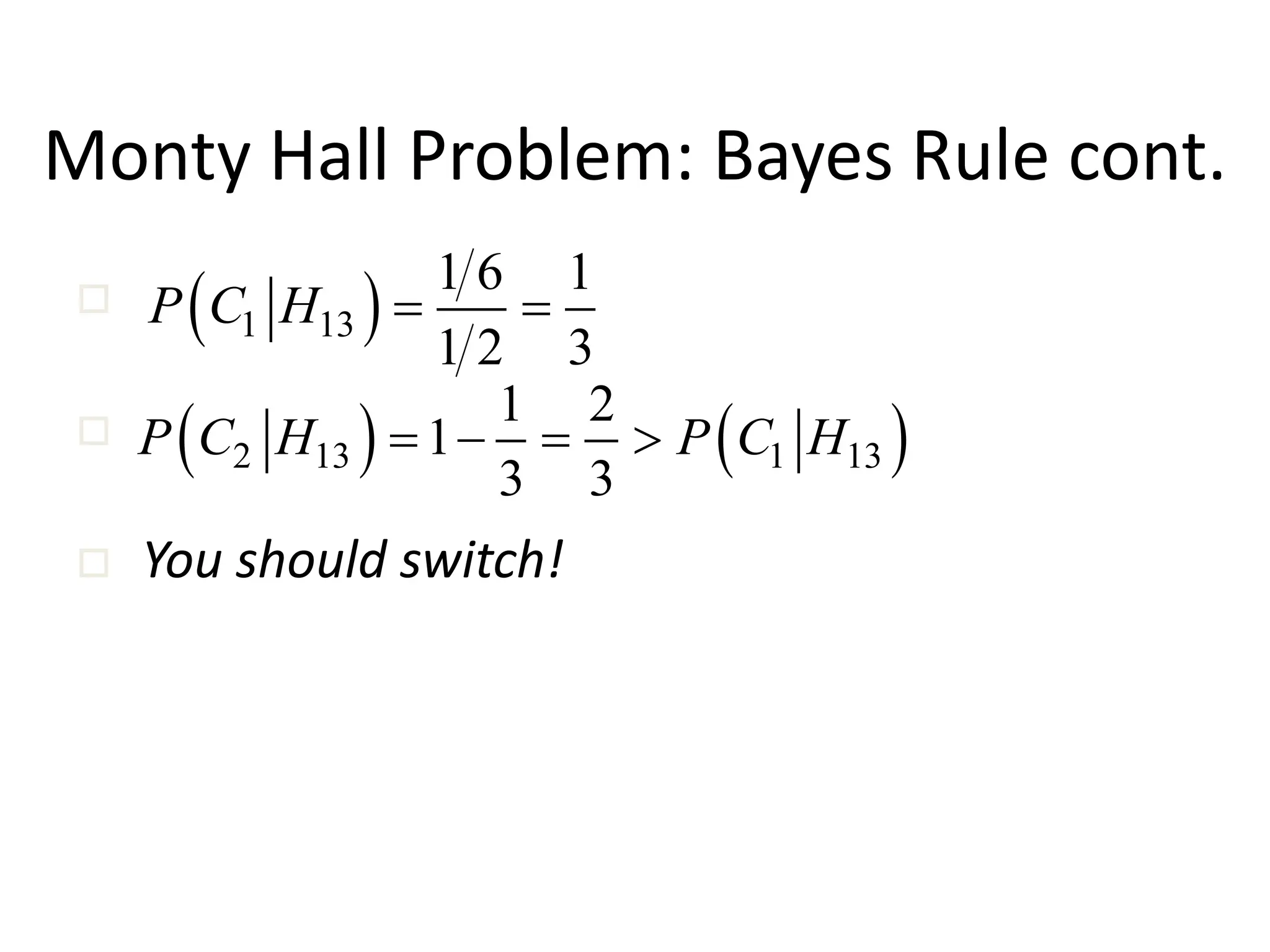
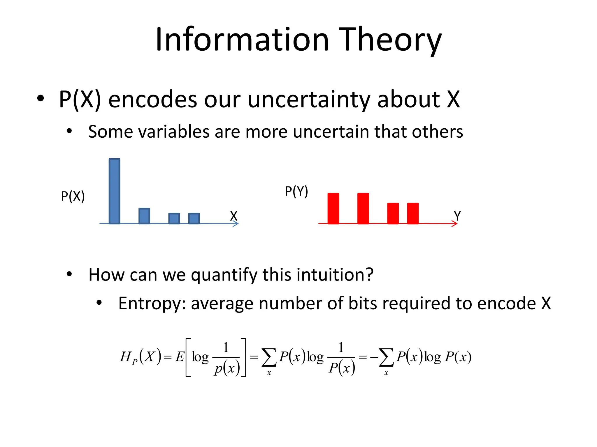

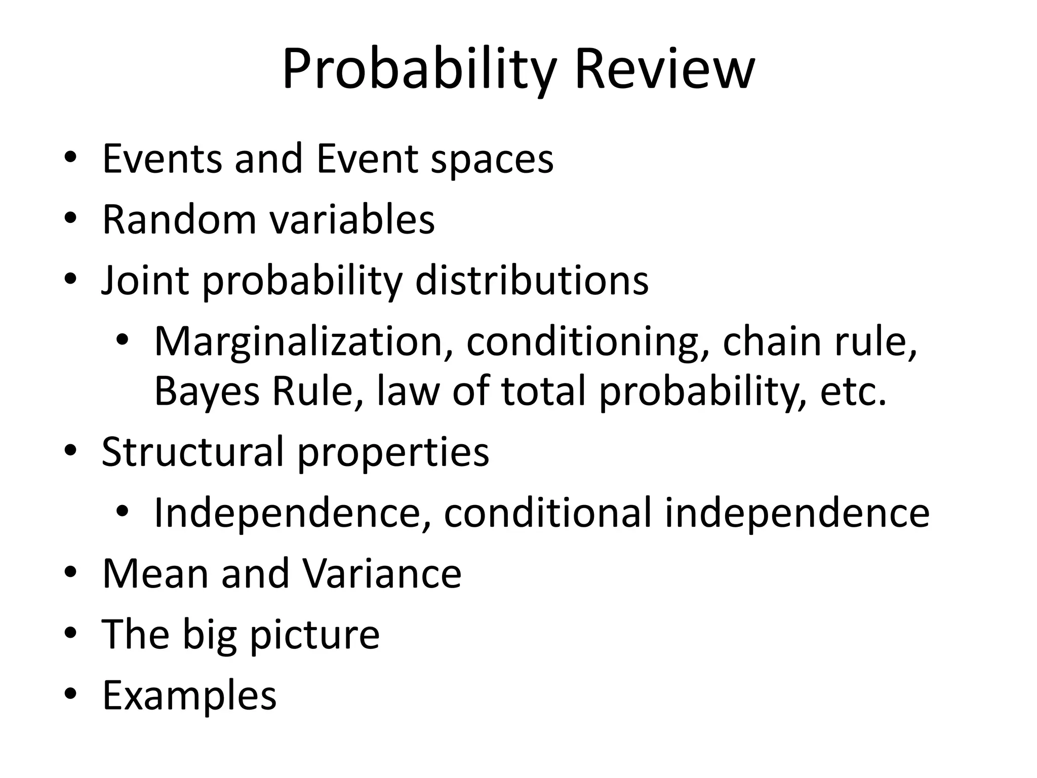
The document covers a comprehensive overview of probability theory, including topics such as events, random variables, joint probability distributions, and key rules like Bayes' rule and the law of total probability. It discusses both discrete and continuous random variables, their probability distributions, and essential concepts such as independence, conditional independence, mean, and variance. Additionally, it touches on practical applications and problems like the Monty Hall problem and information theory, particularly entropy and mutual information.