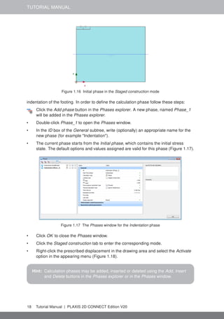
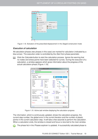
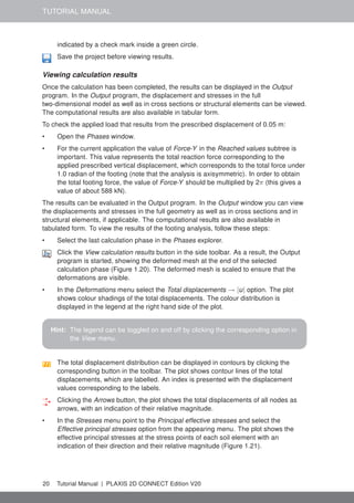
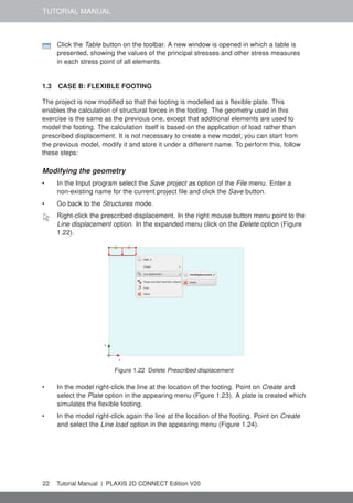
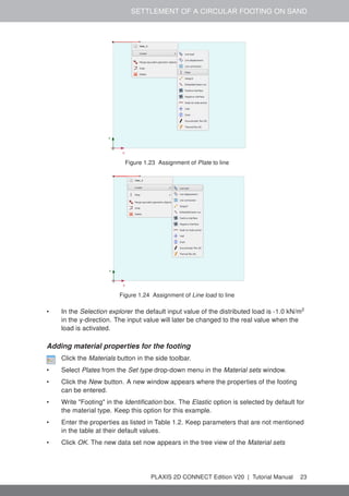
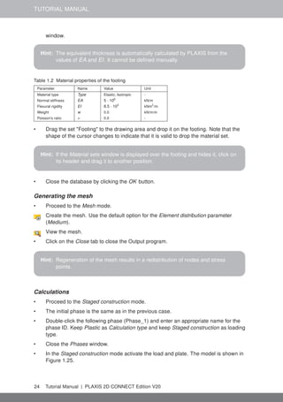
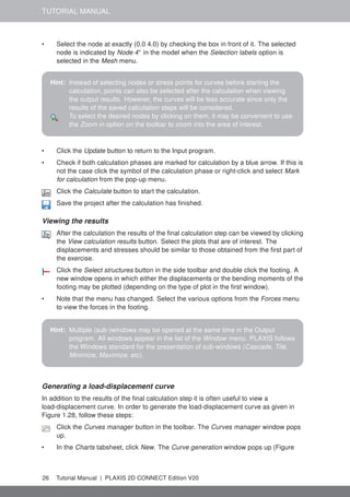
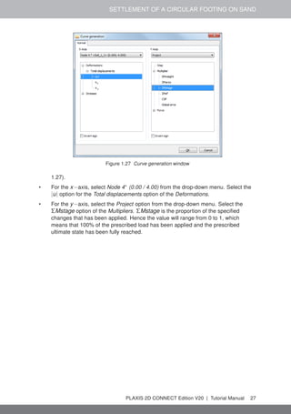
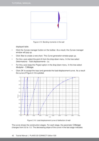
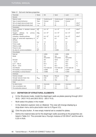
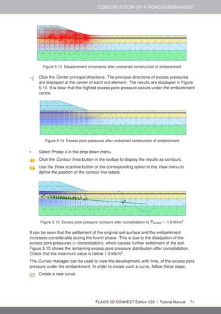
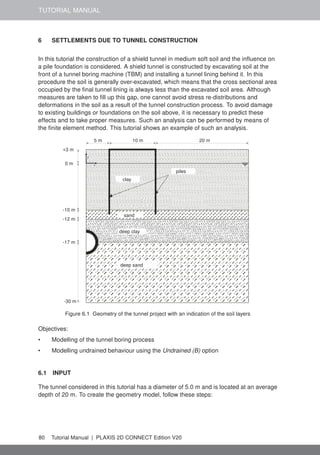
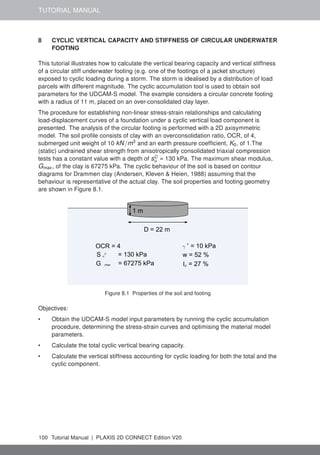
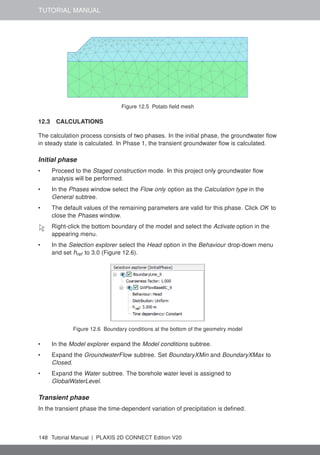
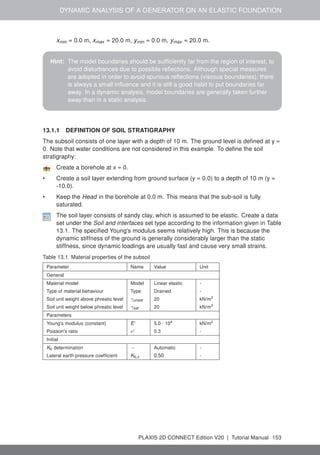
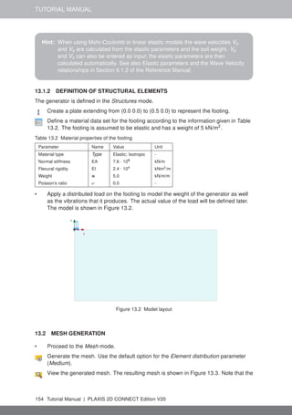
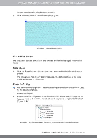
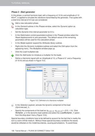
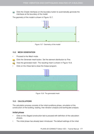
This document is a tutorial manual for PLAXIS 2D that provides step-by-step instructions for 18 geotechnical engineering examples of increasing complexity. The first example models the settlement of a circular footing on sand, with calculations performed for both rigid and flexible footings. It describes how to define the geometry, soil properties, structural elements, generate the mesh, apply loads and boundary conditions, and view the results. Subsequent examples address topics like excavations, embankments, tunnels, foundations, dams and seepage analyses.


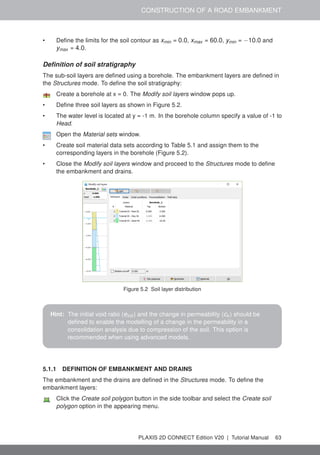

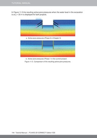
![POTATO FIELD MOISTURE CONTENT
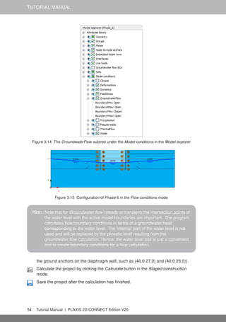
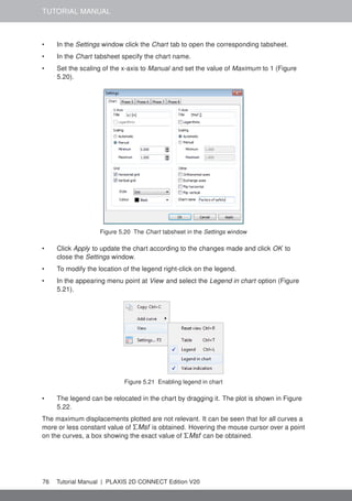
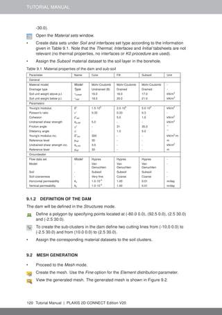
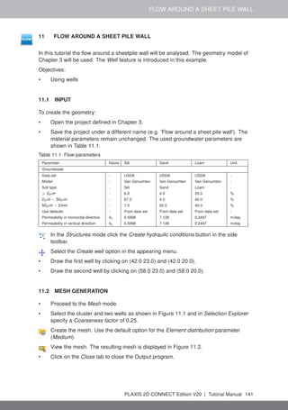
Hint: Note that the conditions explicitly assigned to groundwater flow boundaries
are taken into account. In this tutorial the specified Head will be considered
for the bottom boundary of the model, NOT the Closed condition specified in
the GroundwaterFlow subtree under the Model conditions.
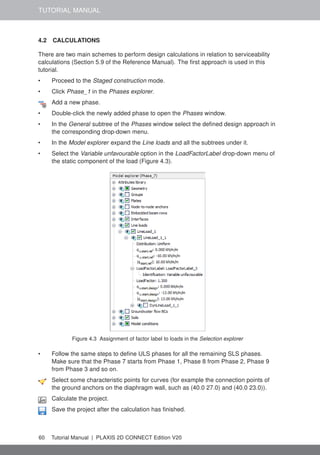
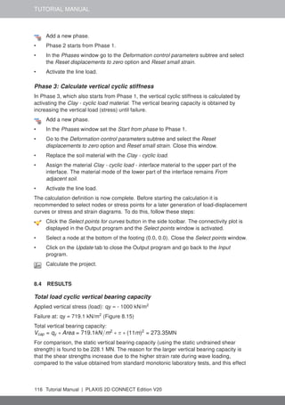
Add a new calculation phase.
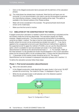
• In General subtree of the Phases window select the Transient groundwater flow as
Pore pressure calculation type.
• Set the Time interval to 15 days.
• In the Numerical control parameters subtree set the Max number of steps stored to
250. The default values of the remaining parameters will be used.
• Click OK to close the Phases window.
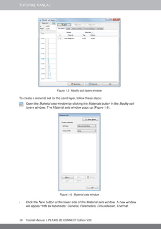
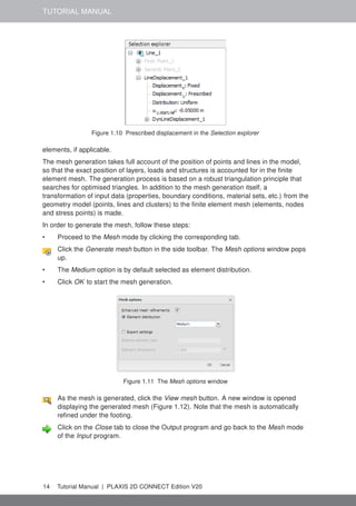
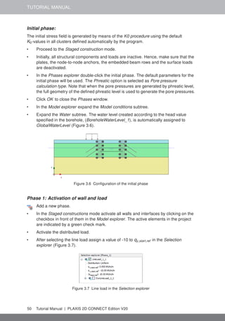
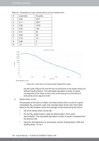
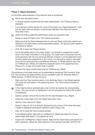
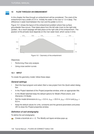
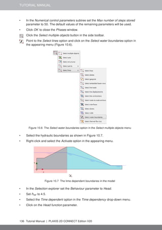
To define the precipitation data a discharge function should be defined.
• In the Model explorer expand the Attributes library subtree.
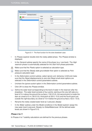
• Right-click on Flow functions and select the Edit option in the appearing menu. The
Flow functions window pops up.
• In the Discharge functions tabsheet add a new function.
• Specify a name for the function and select the Table option in the Signal drop-down
menu.
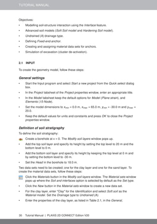
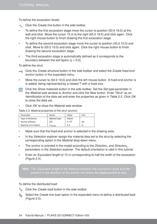
• Click the Add row button to introduce a new row in the table. Complete the data
using the values given in the Table 12.2.
Table 12.2 Precipitation data
ID Time [day] ∆Discharge [m3
/day/m]
1 0 0
2 1 1·10-2
3 2 3·10-2
4 3 0
5 4 -2·10-2
6 5 0
7 6 1·10-2
8 7 1·10-2
9 8 0
10 9 -2·10-2
11 10 -2·10-2
12 11 -2·10-2
13 12 -1·10-2
14 13 -1·10-2
15 14 0
16 15 0
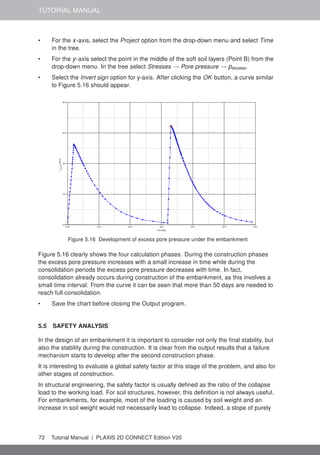
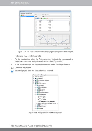
• Figure 12.7 shows the defined function for precipitation. Close the windows by
clicking OK.
• In the Model explorer expand the Precipitation subtree under Model conditions and
activate it. The default values for discharge (q) and condition parameters (ψmin =
PLAXIS 2D CONNECT Edition V20 | Tutorial Manual 149](https://image.slidesharecdn.com/plaxis2dtutorial-211119151715/85/Plaxis-2-d-tutorial-149-320.jpg)
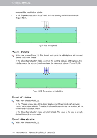

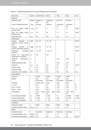
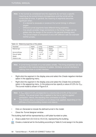
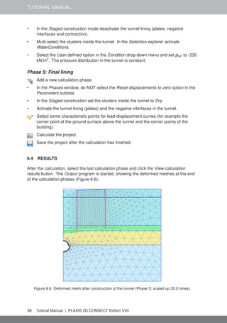
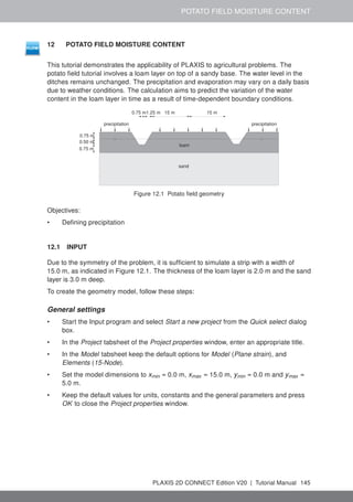
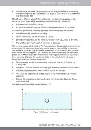
![FREEZE PIPES IN TUNNEL CONSTRUCTION
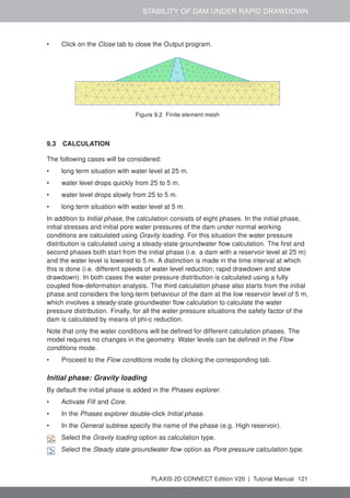
properties of other projects. For more information, refer Section 6.1.6 of the Reference
Manual.
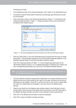
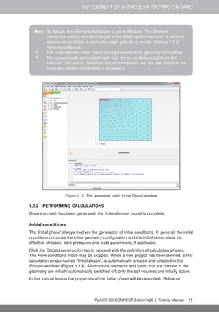
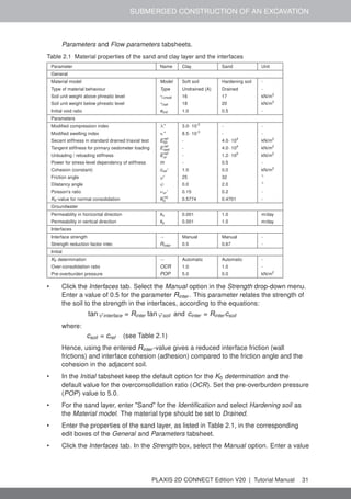
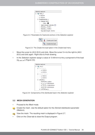
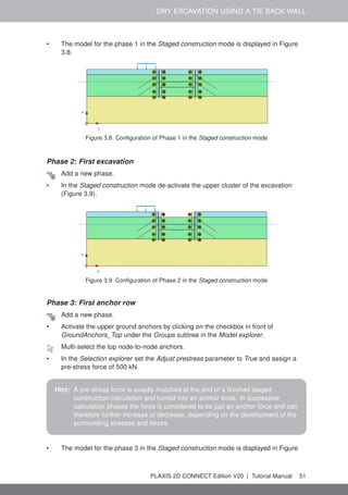
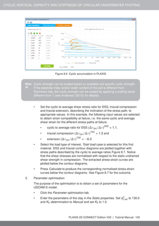
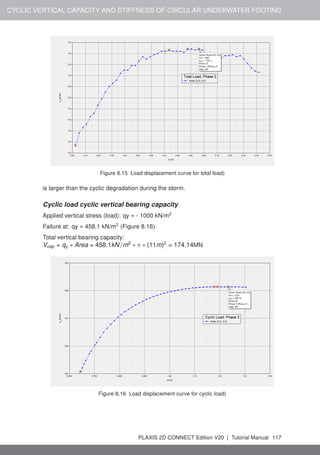
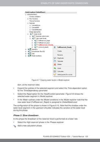
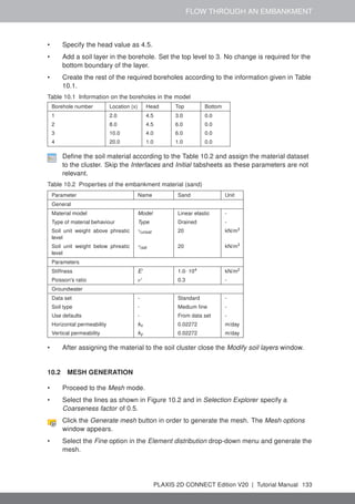
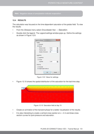
• Click the Thermal tab. Enter the values as given in the Table 17.1.
• Select the option User defined from the drop down menu for Unfrozen water content
at the bottom of the tabsheet.
Add rows to the table by clicking the Add row button to introduce a new row in the
table. Complete the data using the values given in the Table 17.2.
• Enter the values for Interfaces and Initial tabsheets as given in Table 17.1.
• Click OK to close the dataset.
• Assign the material dataset to the soil layer.
Hint: The table can be saved by clicking the Save button in the table. The file must
be given an appropriate name. For convenience, save the file in the same
folder as the project is saved.
Table 17.2 Input for unfrozen water content curve for sand
# Temperature [K] Unfrozen water content [-]
1 273.0 1.00
2 272.0 0.99
3 271.6 0.96
4 271.4 0.90
5 271.3 0.81
6 271.0 0.38
7 270.8 0.15
8 270.6 0.06
9 270.2 0.02
10 269.5 0.00
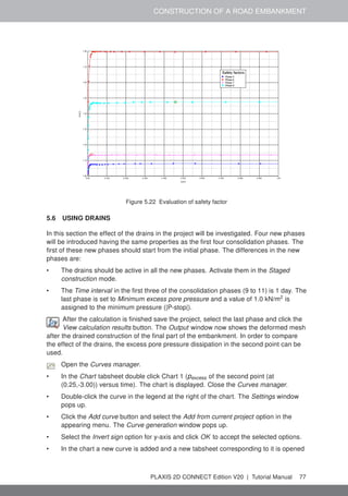
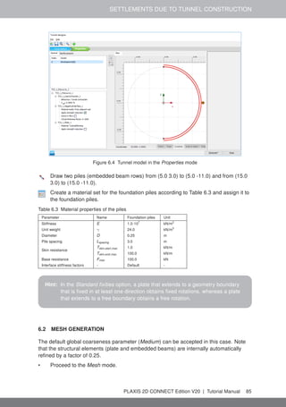
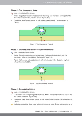
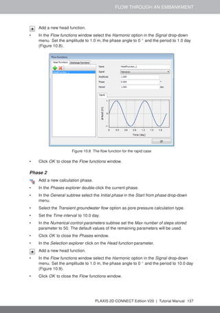
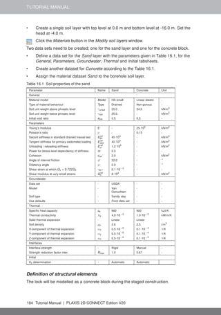
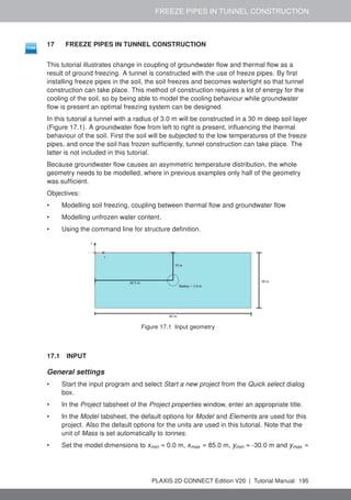
Definition of structural elements
The freeze pipes are modelled by defining lines with a length similar to the freeze pipe
diameter (10 cm), containing a convective boundary condition. For simplicity, in this
tutorial only 12 cooling elements are defined, while in reality more elements may be
implemented in order to achieve a sufficient share of frozen soil.
• Proceed to Structures mode.
Click the Create line button in the side toolbar.
• Click the command line and type "_line 45.141 -13.475 45.228 -13.425". Press
Enter to create the first freezing pipe. For more information regarding command
line, see Section 3.7 of the Reference Manual.
• Similarly create the remaining freeze pipes according to Table 17.3.
Multi select the created lines using the Select lines from the side toolbar.
Right click the selected lines and select Thermal flow BC to create the thermal flow
boundary conditions for the freeze pipes.
PLAXIS 2D CONNECT Edition V20 | Tutorial Manual 197](https://image.slidesharecdn.com/plaxis2dtutorial-211119151715/85/Plaxis-2-d-tutorial-197-320.jpg)

![TUTORIAL MANUAL
19 REFERENCES
[1] Andersen, K.H. (2015). Cyclic soil parameters for offshore foundation design,
volume The 3rd ISSMGE McClelland Lecture of Frontiers in Offshore Geotechnics
III. Meyer (Ed). Taylor & Francis Group, London, ISFOG 2015. ISBN
978-1-138-02848-7.
[2] Andersen, K.H., Kleven, A., Heien, .D. (1988). Cyclic soil data for design of gravity
structures. Journal of Geotechnical Engineering, 517–539.
[3] Jostad, H.P., Torgersrud, Ø., Engin, H.K., Hofstede, H. (2015). A FE procedure for
calculation of fixity of jack-up foundations with skirts using cyclic strain contour
diagrams. City University London, UK.
208 Tutorial Manual | PLAXIS 2D CONNECT Edition V20](https://image.slidesharecdn.com/plaxis2dtutorial-211119151715/85/Plaxis-2-d-tutorial-208-320.jpg)


![Geotechnical Engineering-I [Lec #9: Atterberg limits]](https://cdn.slidesharecdn.com/ss_thumbnails/9-180923180923-thumbnail.jpg?width=640&height=640&fit=bounds)
![Geotechnical Engineering-II [Lec #15 & 16: Schmertmann Method]](https://cdn.slidesharecdn.com/ss_thumbnails/15-181020124920-thumbnail.jpg?width=640&height=640&fit=bounds)


![Geotechnical Engineering-II [Lec #19: General Bearing Capacity Equation]](https://cdn.slidesharecdn.com/ss_thumbnails/19-181123045917-thumbnail.jpg?width=640&height=640&fit=bounds)


![Geotechnical Engineering-I [Lec #21: Consolidation Problems]](https://cdn.slidesharecdn.com/ss_thumbnails/21-180924141121-thumbnail.jpg?width=640&height=640&fit=bounds)


