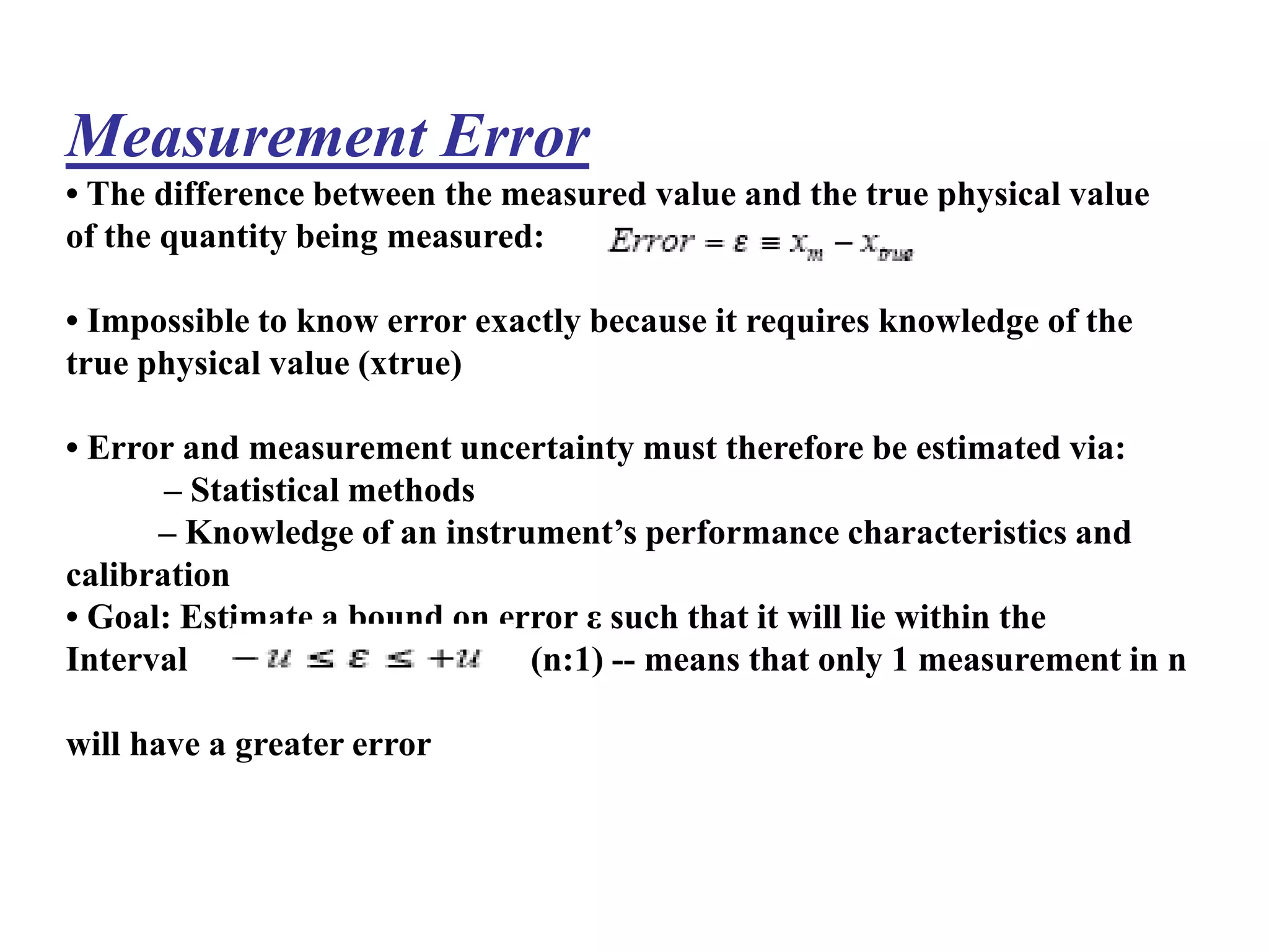
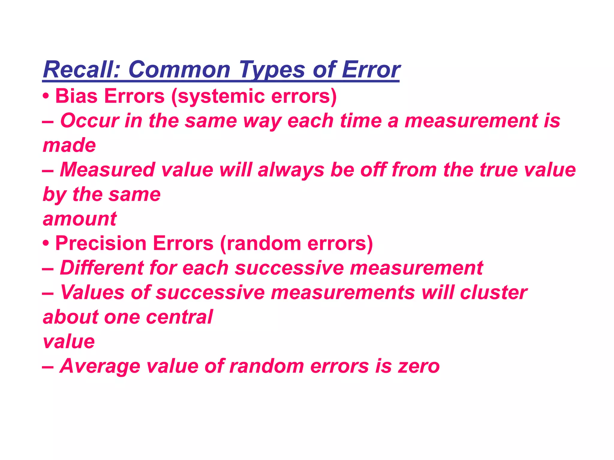
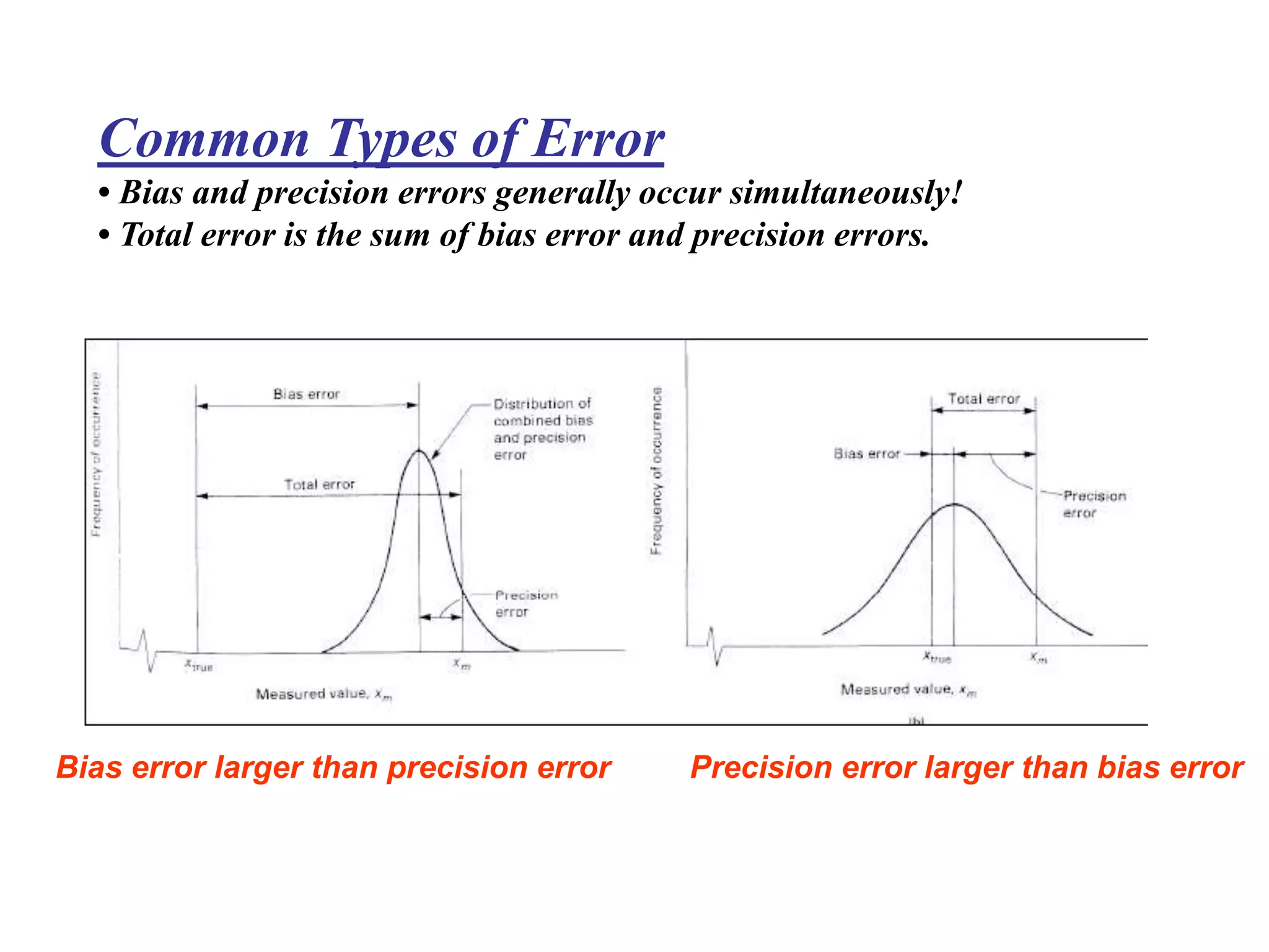
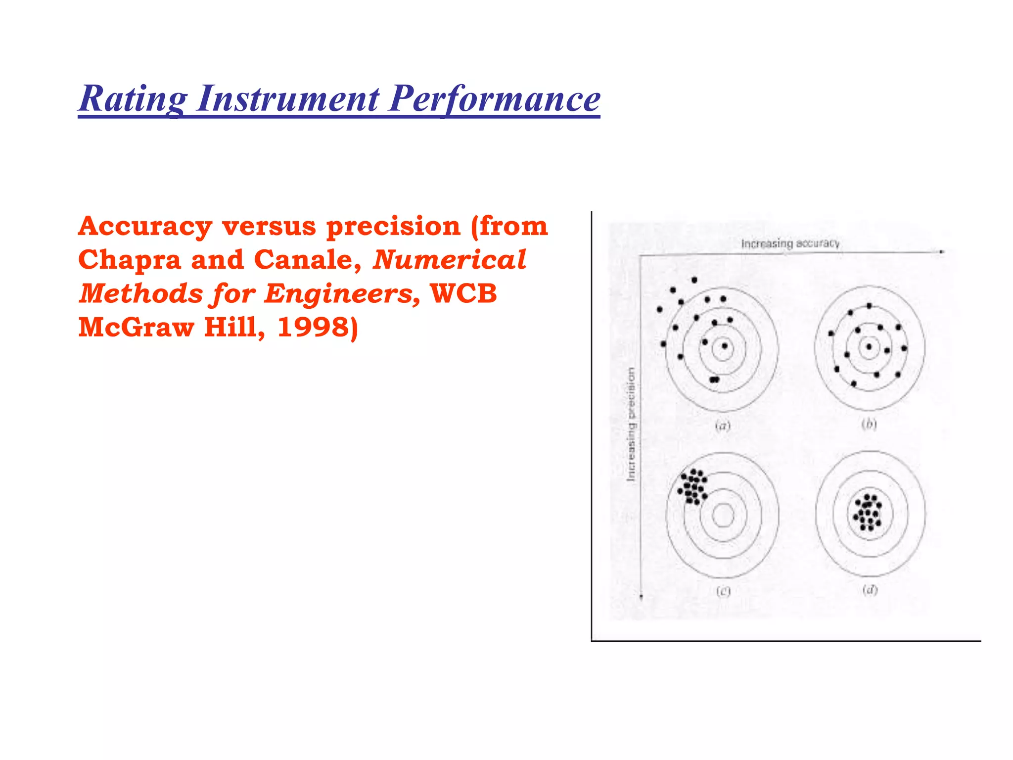
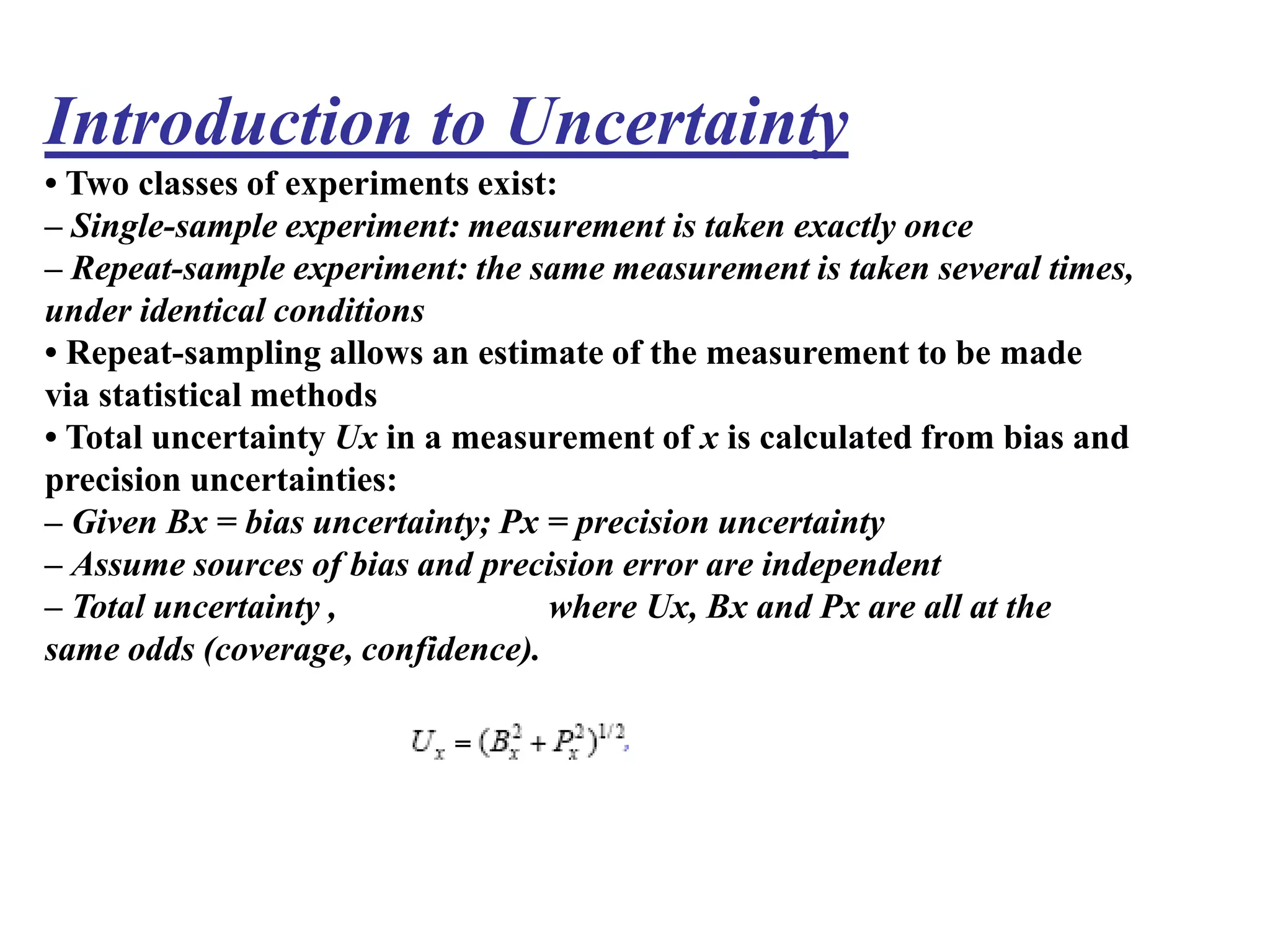
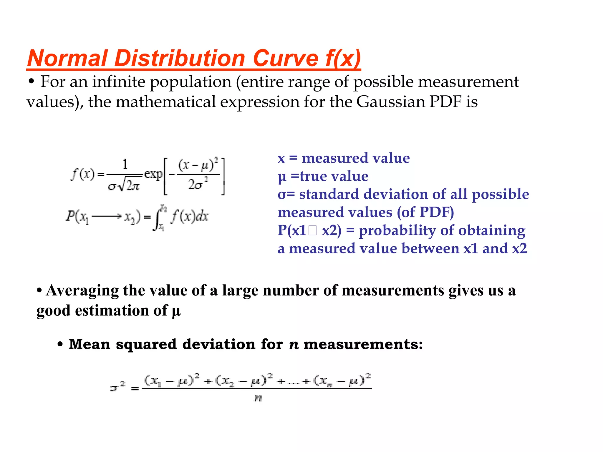
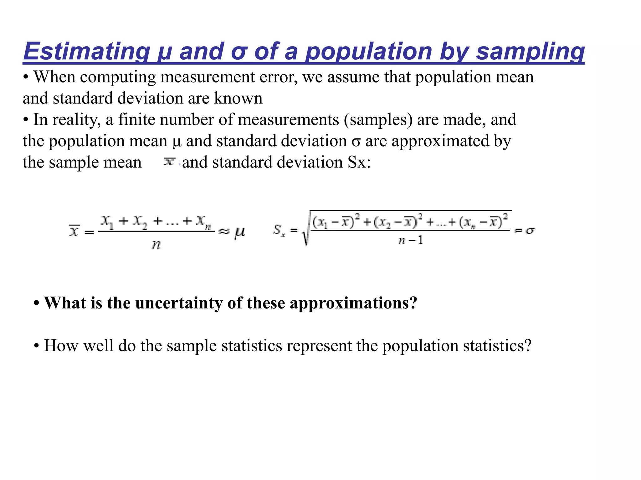
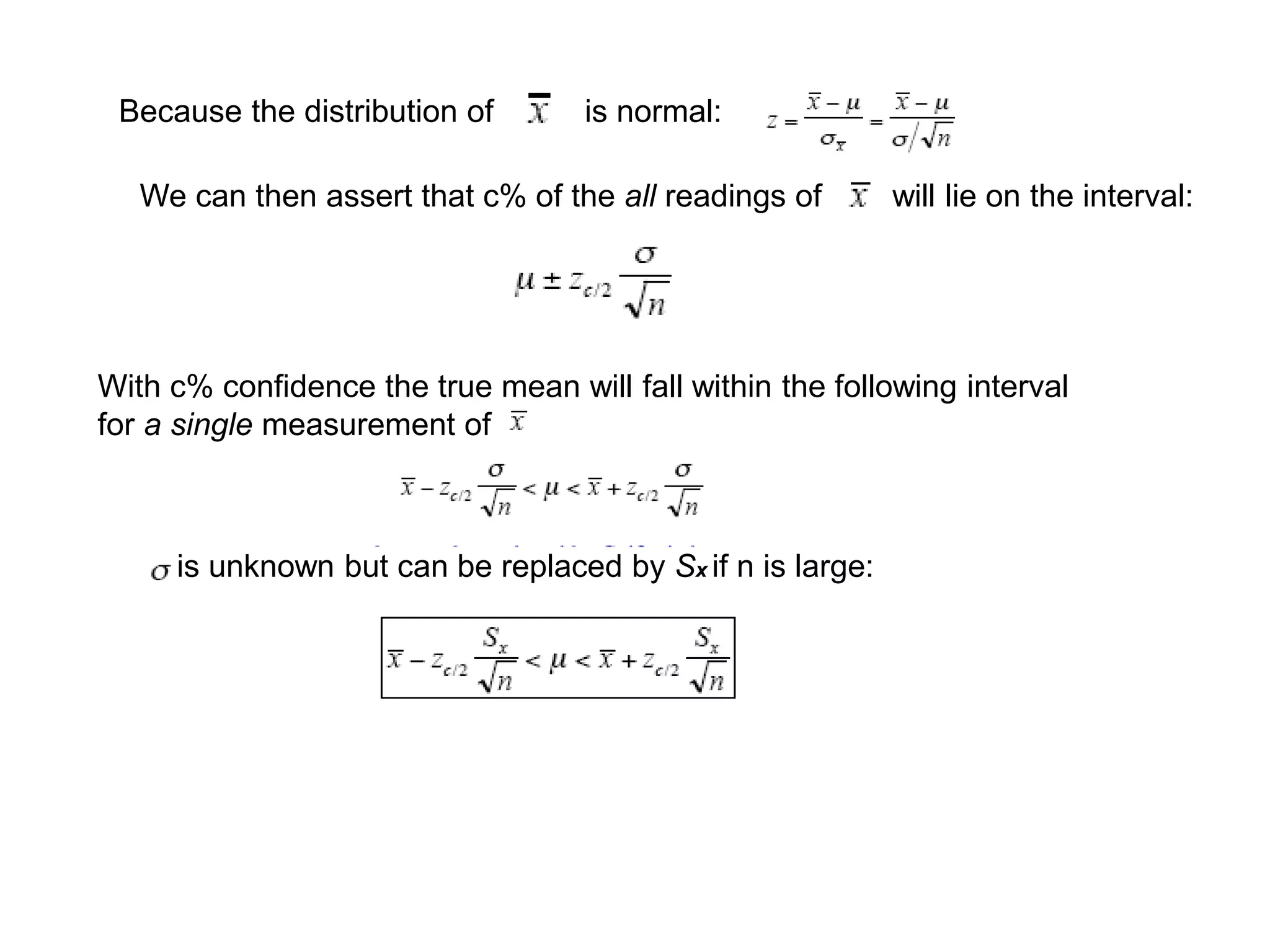
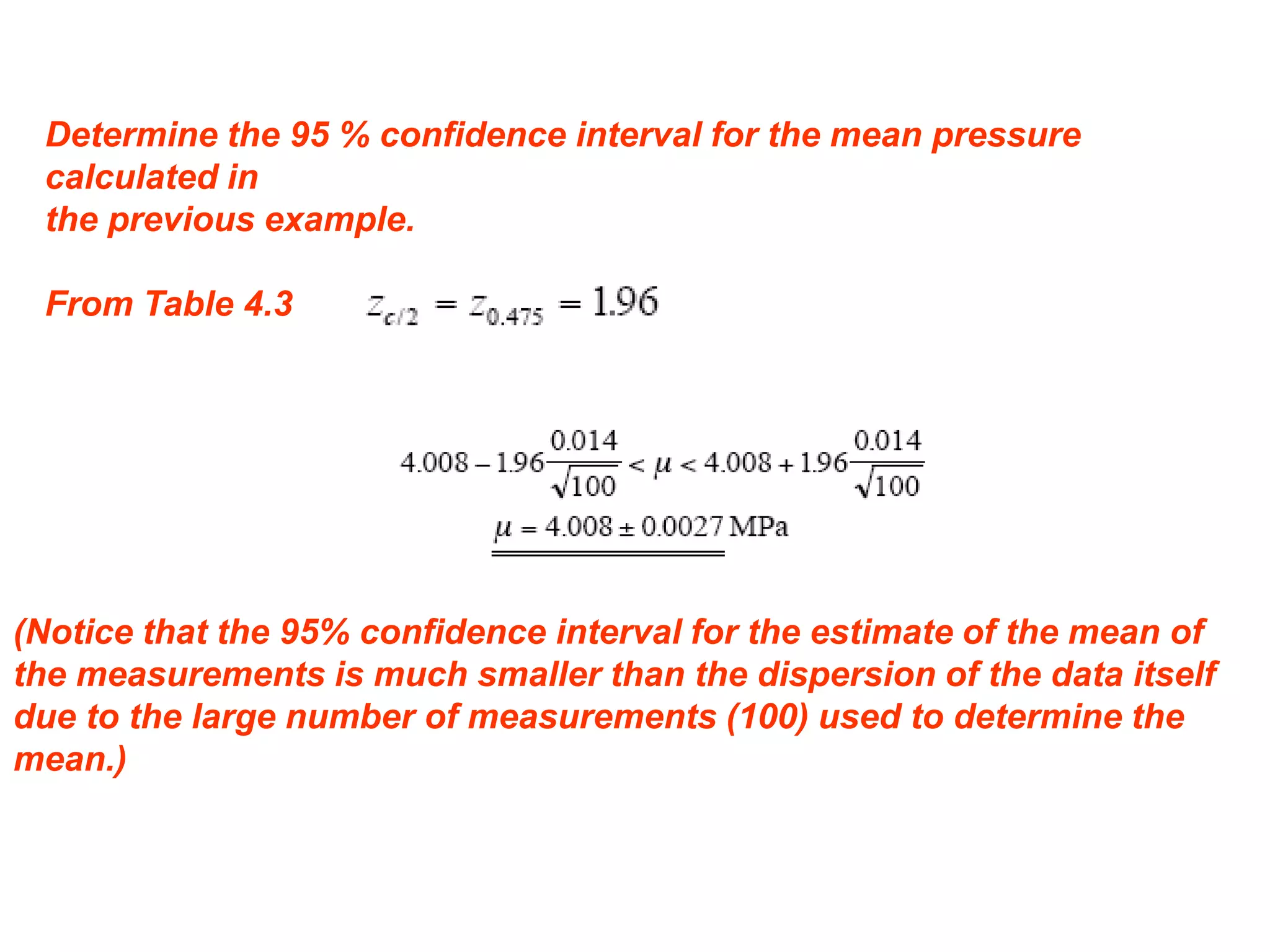
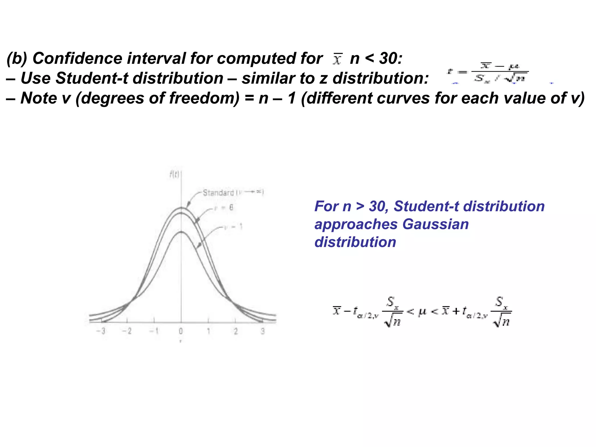
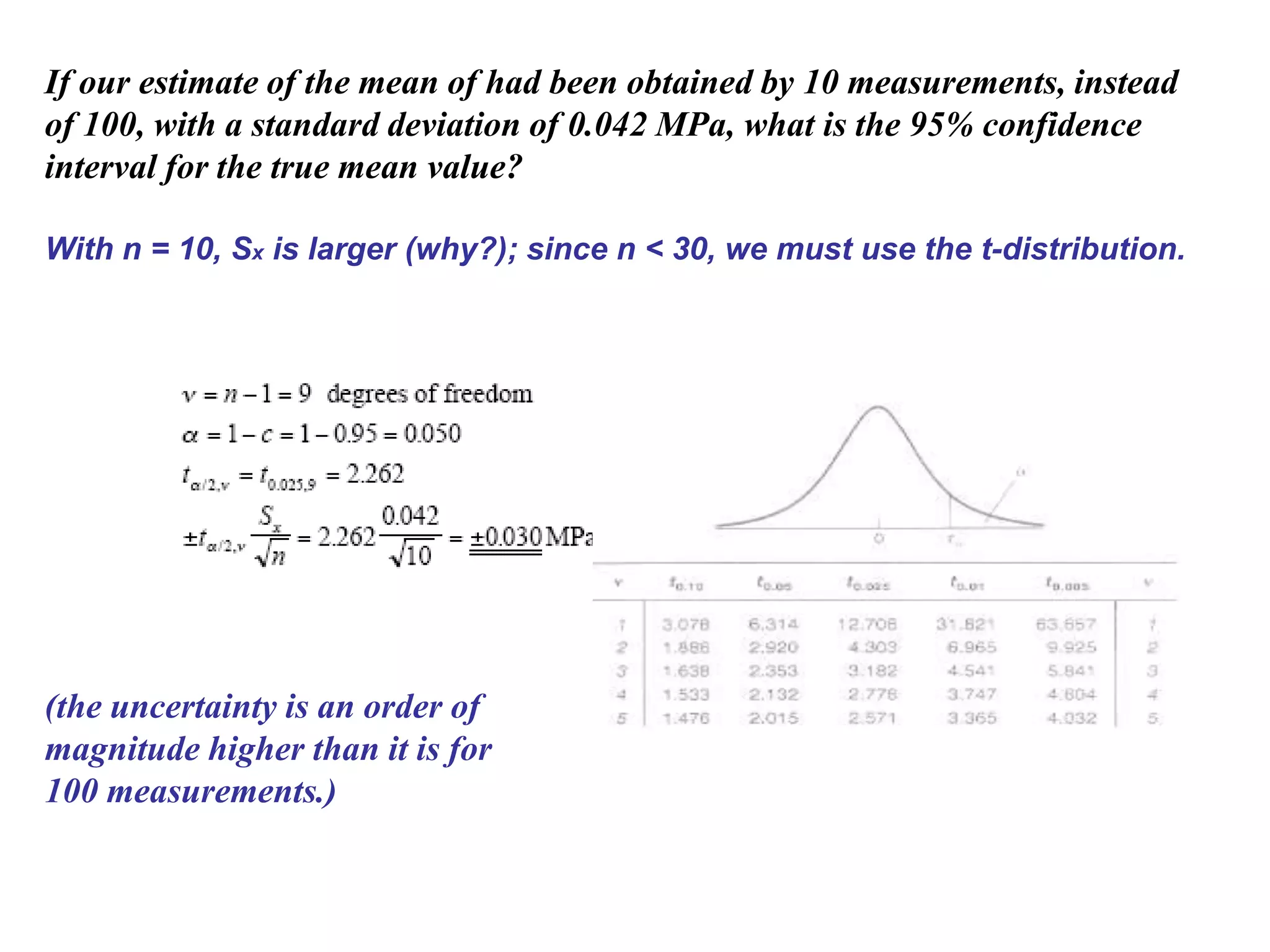
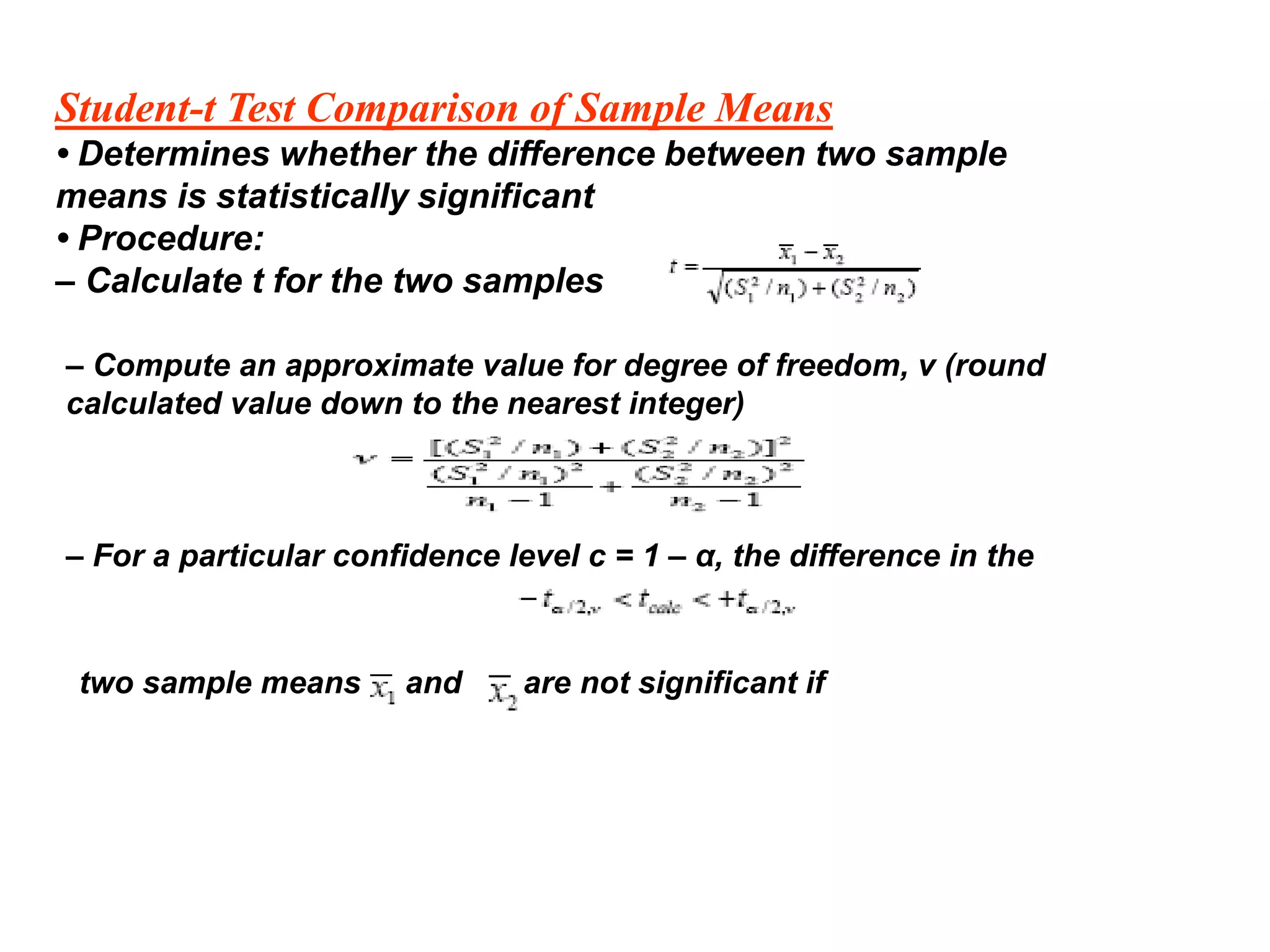
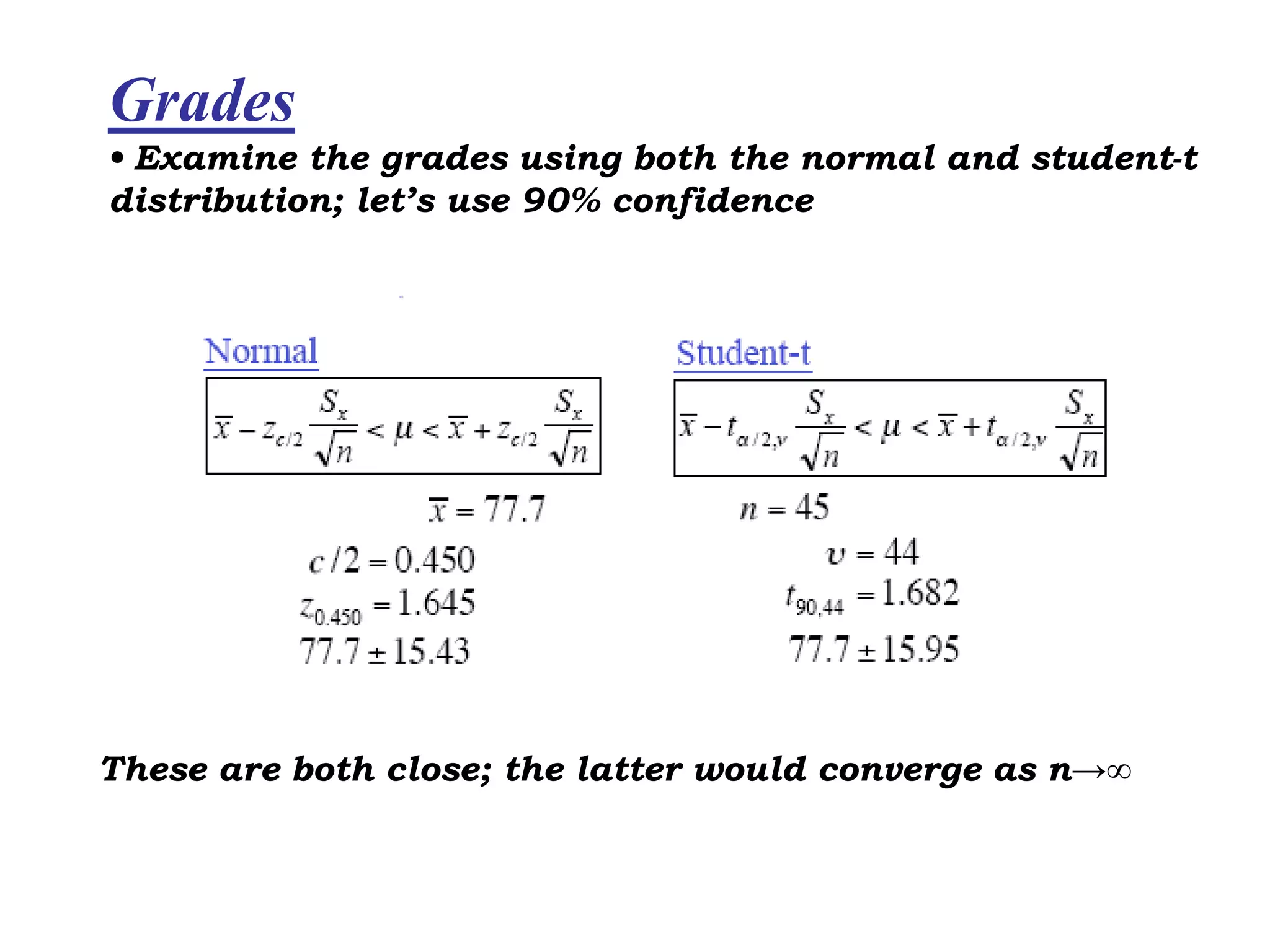
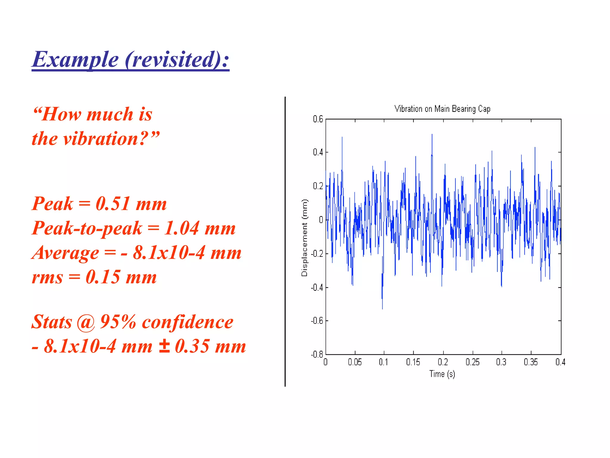
The document discusses measurement error and uncertainty. It explains that total error is the sum of bias error and precision errors. Bias errors are systematic and occur the same way each time, while precision errors are random. Common types of errors include calibration errors, human errors, equipment defects, and environmental factors. Instruments are rated based on their accuracy, precision, resolution, and sensitivity. The normal and standard normal distributions are used to model measurement uncertainty and determine confidence intervals for means and deviations based on sample size and coverage percentage.

1. Probability &
Statistics
ME 310 – Engineering
Experimentation I

2. Example:
Consider again
the question “how
much is the
vibration?”
• Peak (max) value?
• Average value?
• “Effective” value?
• Some statistical measure?
• Spectral (frequency) composition? Been there, done that.

3. Measurement Error
• The difference between the measured value and the true physical value
of the quantity being measured:
• Impossible to know error exactly because it requires knowledge of the
true physical value (xtrue)
• Error and measurement uncertainty must therefore be estimated via:
– Statistical methods
– Knowledge of an instrument’s performance characteristics and
calibration
• Goal: Estimate a bound on error ε such that it will lie within the
Interval (n:1) -- means that only 1 measurement in n
will have a greater error

4. Recall: Common Types of Error
• Bias Errors (systemic errors)
– Occur in the same way each time a measurement is
made
– Measured value will always be off from the true value
by the same
amount
• Precision Errors (random errors)
– Different for each successive measurement
– Values of successive measurements will cluster
about one central
value
– Average value of random errors is zero

5. Common Types of Error
• Bias and precision errors generally occur simultaneously!
• Total error is the sum of bias error and precision errors.
Bias error larger than precision error Precision error larger than bias error

6. Classification of Errors
• Bias or Systemic
– Calibration errors (most common; may be zero-offset or scale)
– Consistently recurring human errors
– Certain errors caused by defective equipment (e.g. incorrect
gradation)
– Loading errors (recall: measurement changes the system being
measured)
– Limitations of system resolution
• Precision or Random
– Certain human errors
– Disturbance to equipment (movement, re-zero)
– Fluctuating experimental conditions (temperature, vibration)
– Insufficient measuring-system sensitivity

7. Classification of Errors
• Illegitimate errors: Errors not due to the equipment
– Blunders and mistakes during an experiment
– Computational errors made after an experiment
• Sometimes bias/sometimes precision errors
– Backlash, friction, hysteresis
– Calibration drift; variation in test or environmental
conditions
– Variations in procedure among different experimenters
– Variations caused by performing the same experiment
using
different equipment.

8. Classification of Errors
• Hysteresis; note loading and
unloading portion of curves
• Measured values of the speed
of
light: what can we tell from
these data?

9. Rating Instrument Performance
• Accuracy
– Difference between measured and true values
– Often specified as a maximum error; odds that an error will not exceed
that maximum value are generally not specified (bad!)
• Precision: Difference between the instrument’s reported values
during
repeated measurements of the same quantity
• Resolution
– The smallest increment of change in the measured value that can be
determined from the instrument’s readout scale
– The resolution of an instrument is generally the same or smaller than
the
precision
• Sensitivity: Change of an instrument or transducer’s output per unit
change in measured quantity (e.g. 5 volts/division on an oscilloscope)

10. Rating Instrument Performance
Accuracy versus precision (from
Chapra and Canale, Numerical
Methods for Engineers, WCB
McGraw Hill, 1998)

11. Introduction to Uncertainty
• Two classes of experiments exist:
– Single-sample experiment: measurement is taken exactly once
– Repeat-sample experiment: the same measurement is taken several times,
under identical conditions
• Repeat-sampling allows an estimate of the measurement to be made
via statistical methods
• Total uncertainty Ux in a measurement of x is calculated from bias and
precision uncertainties:
– Given Bx = bias uncertainty; Px = precision uncertainty
– Assume sources of bias and precision error are independent
– Total uncertainty , where Ux, Bx and Px are all at the
same odds (coverage, confidence).

12. Estimation of Precision Uncertainty
• Error Distribution: Characterizes the probability that an error of a
given size will occur during repeat-sample experiments
• Probability: an expression of the likelihood of a particular event taking
place, measured with reference to all possible events
• The probability density function (PDF) for the entire population of
possible precision error values is generally assumed to be Gaussian
(normal, bell-shaped)
• Note that PDFs other than Gaussian are possible (see Table 4.2 in text)
• Since total precision error is random, each individual measurement in
the sample will have a distinct error whose likelihood of occurrence
(roughly) decreases with size

13. Normal Distribution Curve f(x)
• For an infinite population (entire range of possible measurement
values), the mathematical expression for the Gaussian PDF is
x = measured value
μ =true value
σ= standard deviation of all possible
measured values (of PDF)
P(x1 x2) = probability of obtaining
a measured value between x1 and x2
• Averaging the value of a large number of measurements gives us a
good estimation of μ
• Mean squared deviation for n measurements:

14. Normal Distribution Curve f(x)
More precise data have lower values of standard deviation;
Amplitude is given by

15. Normal Distribution Curve f(x)
Assuming normal distribution, “error level” can be expressed
in terms of standard deviation (σ)
(Note the commonly touted “six-sigma” criteria used in industry is 3.4
“defects” per million events. See www.ge.com/sixsigma)

16. Standard Normal Distribution f(z)
• A simple transform allows values of f(x) to be normalized and expressed as
f(z):
• Values of the normal curve range from 0 – 1, and are often found via table

17. Estimating μ and σ of a population by sampling
• When computing measurement error, we assume that population mean
and standard deviation are known
• In reality, a finite number of measurements (samples) are made, and
the population mean μ and standard deviation σ are approximated by
the sample mean and standard deviation Sx:
• What is the uncertainty of these approximations?
• How well do the sample statistics represent the population statistics?

18. Standard Normal Distribution f(z)
• A simple transform collapses all f(x)’s to to a single function f(z):

19. Standard Normal Distribution f(z)
• Total area under the normal curve = 1.0. Area between z = 0 and any
other
value can be found using Table 4.3

20. Example
• Statement: From long-term plant-maintenance data, it is observed that
the flow pressure taken at a certain point has a mean value of 303 psi with
a standard deviation of 33 psi. What is the probability that the a
particular measured pressure will exceed 350 psi (during normal
operation):
• Solution: want area under curve corresponding to p > 350 psi
– Calculate z = (x-μ)/σ = (350-303)/33 = 1.42
– Want P(z > 1.42) = 1 - P(z < 1.42) = 1 - 0.500 - P(0 < z < 1.42)
= 0.5 - 0.4222 = 0.0778
=7.8%

21. • When computing measurement error, we assume that the population
mean μ and standard deviation σ are known
• In reality, a finite number of measurements (samples) are made, and
the population mean μ and standard deviation σ are approximated by
the sample mean and sample standard deviation Sx:
Estimating μ and σ of a population by sampling
• What is the uncertainty of these approximations?
• How well do the sample statistics represent the population
statistics?
• Note that each set of measurements will yield a distinct and Sx

22. Estimating μ and σ of a population by sampling
• Example: Pressure data plotted using a histogram
• Number of results in each bin is the number of readings falling in
interval of +/- 0.005 MPa centered about the listed pressure
• Histogram shows that the data approximate a Gaussian distribution

23. Example (cont.)
1. What is the interval that is likely to contain 95 % of the readings?
2. What is the likelihood that the pressure will deviate more than 1 % from
the desired of 4.00 Mpa?
• Assuming the distribution of pressure measurements is normal and that the sample
mean
and sample standard deviation are equal to the population mean and standard deviation,
i.e
Table 3.1 (based on the z-table) may be used to answer these questions.
From Table 4.3 (unity standard deviation), the area corresponding
to z = 2.86 is 0.4979; the chance that the pressure is greater than
4.04 MPa is therefore 21 out of 5000 or one chance in 238.

24. Estimating μ and σ of a population by sampling
• There are two possibility choices when determining the confidence
internal: (a) normal distribution for many measurements and (b) student-t
for smaller measurement sets
(a) Confidence interval for computed using many measurements:
– Answers the question: what is the estimate for the uncertainty in using
An to approximate the true population mean μ?
– The set of all obtained (mean calculated from each sample) will
show a Gaussian distribution about the true population mean μ, as
long as n is large for each sample
show a Gaussian distribution about the true population mean μ, as
long as n is large for each sample
– The standard deviation of the sample means is
(Central Limit Theorem of statistics)

25. Because the distribution of is normal:
We can then assert that c% of the all readings of will lie on the interval:
With c% confidence the true mean will fall within the following interval
for a single measurement of
is unknown but can be replaced by Sx if n is large:

26. Determine the 95 % confidence interval for the mean pressure
calculated in
the previous example.
From Table 4.3
(Notice that the 95% confidence interval for the estimate of the mean of
the measurements is much smaller than the dispersion of the data itself
due to the large number of measurements (100) used to determine the
mean.)

27. (b) Confidence interval for computed for n < 30:
– Use Student-t distribution – similar to z distribution:
– Note ν (degrees of freedom) = n – 1 (different curves for each value of ν)
For n > 30, Student-t distribution
approaches Gaussian
distribution

28. If our estimate of the mean of had been obtained by 10 measurements, instead
of 100, with a standard deviation of 0.042 MPa, what is the 95% confidence
interval for the true mean value?
With n = 10, Sx is larger (why?); since n < 30, we must use the t-distribution.
(the uncertainty is an order of
magnitude higher than it is for
100 measurements.)

29. Student-t Test Comparison of Sample Means
• Determines whether the difference between two sample
means is statistically significant
• Procedure:
– Calculate t for the two samples
– Compute an approximate value for degree of freedom, ν (round
calculated value down to the nearest integer)
– For a particular confidence level c = 1 – α, the difference in the
two sample means and are not significant if

30. Grades
• Examine the grades using both the normal and student-t
distribution; let’s use 90% confidence
These are both close; the latter would converge as n→∞

31. Example (revisited):
“How much is
the vibration?”
Peak = 0.51 mm
Peak-to-peak = 1.04 mm
Average = - 8.1x10-4 mm
rms = 0.15 mm
Stats @ 95% confidence
- 8.1x10-4 mm ± 0.35 mm

32. Bias and Single-Sample Uncertainty
• Provides no direct evidence of either bias error’s
magnitude or its presence
• Can only be found definitively by repeating measurement
on another piece of equipment, which is seldom done
• Estimated by examining
– Applicability of handbook or manufacturers values for physical
properties used
– Calibration; standards used during calibration procedure

33. Approaches for Minimizing Experimental Error
• Best time to minimize error is in experiment’s design stage
• Perform an uncertainty analysis before an experiment is built
• General precautions to observe during the design of an experiment
– Avoid approaches that require two large numbers to be measured in
order
to determine the small difference between them
– Design experiments or sensors that amplify the signal strength in
order to
increase sensitivity
– Build null designs where the output is measured as a change from
zero
(reduces bias and precision error – e.g. Wheatstone Bridge)
– Avoid experiments in which large correction factors are required
– Attempt to minimize the influence of measuring system on the
measurand
– Calibrate entire systems, rather than individual components, to
minimize
calibration-related bias error

34. Linear Regression and Best Fits to Data
• It’s often easier to interpret data when they are presented as a
line;
straight-line transformations are summarized in Chapter 4
• Once the data has been linearized and plotted, a line may be fit
by
– “eye-balling” the data
– Method of least squares
• Best fit means just that – all points will not be on the line
• Goodness of fit is evaluated using the correlation coefficient: r2
closer
to 1 implies better fit
• Deviations from the line are often due to precision error
• Packages such as Excel, MathCAD and MATLAB contain line-
fitting
software

35. Note to students
• Goodness of fit is evaluated by comparing the
histogram
with the Gaussian distribution plotted using the sample
mean and standard deviation. Other methods discussed
in
Chapter 4 are not covered.
• The Chi-Squared Distribution is not covered in ME 310.
• The notation for ta,b in the Student-t distribution vary
from
text to text; just be aware of the definitions of c, α, and υ
and you can’t go wrong!