Instrumentation Lecture

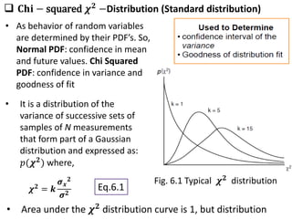
1.  𝐂𝐡𝐢 − squared 𝝌𝟐
−Distribution (Standard distribution)
• It is a distribution of the
variance of successive sets of
samples of N measurements
that form part of a Gaussian
distribution and expressed as:
𝑝(𝝌𝟐) where,
𝝌𝟐
= 𝒌
𝝈𝒙
𝟐
𝝈𝟐
Fig. 6.1 Typical 𝝌𝟐 distribution
• Area under the 𝝌𝟐
distribution curve is 1, but distribution
Eq.6.1
• As behavior of random variables
are determined by their PDF’s. So,
Normal PDF: confidence in mean
and future values. Chi Squared
PDF: confidence in variance and
goodness of fit

2. 𝜎𝑥
2 variance of a sample of N measurements.
𝜎2
is the variance of the infinite data set.
𝑘 is a constant known as the number of degrees of freedom
and is equal to 𝑁 − 1. The shape of the 𝜒2
distribution
depends on the value of 𝑘 as shown in Fig. 6.1
is not symmetrical; it tends toward symmetrical shape of a
Gaussian distribution when 𝑘 becomes very large
• The 𝜒2
distribution is to predict the variance 𝝈𝟐
of an infinite
data set, given the measured variance 𝜎𝑥
2
of a sample of 𝑁
measurements.
• The magnitude of this expected variation depends on level of
“random chance” which is normally expressed as a level of
significance, 𝜶

3. 𝑃 χ𝟐
1−𝛼
2
≤ χ𝟐 ≤ χ𝟐
𝛼
2
= 1 − 𝛼
the area of the curve to the
right of χ𝟐
𝛼 is 𝛼 and that to
the left is (1 − 𝛼).
e.g. for a level of significance 𝛼 = 0.05, there is 95% probability
(95% confidence level) that χ𝟐 lies χ𝟐
0.975 χ𝟐
0.025.
Eq.6.2
Probability of (1 − 𝛼)%
• Precision interval for
variance with probability
𝑃and particular level of
significance 𝜶 can be
expressed as:

5. 𝑃
𝑘 𝜎𝑥
2
χ𝟐
1−𝛼
2
≥ 𝜎𝟐
≥
𝑘𝜎𝑥
2
χ𝟐
𝛼
2
= 1 − 𝛼
Eq.6.1
Substituting into Eq.6.2 and simplify:
• The range, where predictions of the true variance and standard
deviation lie, is wide due to small number of measurements in the
sample.
• Therefore, larger sample size should be used for prediction of the
variance of whole population that the sample is drawn from.
Eq.6.3
The length of each rod in a sample of 10 brass rods is measured, and
the variance of the length measurement in the sample is found to be
16.3 mm. Estimate the true variance and standard deviation for the
whole batch of rods from which the sample of 10 was drawn, expressed
to a confidence level of 95%.
Numerical Problem P6.1 :

6. ✔ Solution is done in class.
The length of a sample of 25 bricks is measured and the variance of the
sample is calculated as 6.8 mm. Estimate the true variance for the whole
batch of bricks from which the sample of 25 was drawn, expressed to
confidence levels of (a) 90%, (b) 95%, and (c) 99%.
Numerical Problem P 6.2:
✔ Solution is done in class.
 Testing Goodness of Fit (to a Gaussian Distribution)
• Degree to which a data set fits a Gaussian distribution should
always be tested before any analysis is carried out; which can
be done in the following three ways:
(i) Inspecting the shape of histogram
(ii) Using a normal probability plot

7. (iii) The χ𝟐
-test (more formal method whether data set follow
the Gaussian distribution)
 Inspecting the Shape of Histogram
• Plot a histogram and look for a “bell shape”
• For a Gaussian distribution, there must always be approximate
symmetry about the center line of the histogram.
 Using a Normal Probability Plot
• A normal probability plot (straight line when data distribution
is Gaussian) is drawn by dividing data values into a number of
ranges and plotting the cumulative probability of summed data
frequencies against data values on special graph paper.

8. • Careful judgmental experience is required to decide whether
the line is straight enough to indicate a Gaussian distribution.
Suppose that the length measurements of a steel bar are: 409
406 402 407 405 404 407 404 407 407 408 406 410 406 405 408
406 409 406 405 409 406 407
Range 401.5
to
403.5
403.5
to
405.5
405.5
to
407.5
407.5
to
409.5
409.5
to
411.5
No. data in Range 1 1 5 11 5 1
Cumulative No. of Data
Items
1 6 17 22 23
Cumulative No. of Data
Items as % age
4.3 26.1 73.9 95.7 100.0

9.  The χ𝟐
-test
• More formal method for testing whether data follow a Gaussian
distribution.
• The data is divided into p equal width bins like it is done to
construct a histogram & count the number of measurements
𝑛𝑖 in each bin.
• χ𝟐
-test provides
measure of the
discrepancy between
measured variation &
variation predicted by
your PDF.

10. χ𝟐
=
(𝑛𝑖−𝑛𝑖
′)2
𝑖
𝑛𝑖
′ for 𝑖 = 1,2, … . , p Eq. (6.4)
Lower χ𝟐
better fit
𝑛𝑖: No. of observations
𝑛𝑖
′
: Expected # of observations
p: No. of bins
• The expected number of measurements 𝑛𝑖
′
in each bin for a
Gaussian distribution is also calculated.
• Check to ensure that at least 80% of the bins have a data count
> min(𝑛𝑖 & 𝑛𝑖
′
). The min. number is taken to be 4.
• A χ𝟐
value is calculated for the data according to the following
formula:
• The expected value is read off from the χ𝟐
distribution table
for the specified confidence level and comparing this
expected value with that calculated in Eq. (6.4).

11. A sample of 100 pork pies produced in a bakery is taken, and the mass of
each pie (grams) is measured. Apply the χ𝟐-test to examine whether the
data set formed by the set of 100 mass measurements shown below
conforms to a Gaussian distribution.
487 504 501 515 491 496 482 502 508 494 505 501 485 503 507 494 489
501 510 491 503 492 483 501 500 493 505 501 517 500 494 503 500 488
496 500 519 499 495 490 503 500 497 492 510 506 497 499 489 506 502
484 495 498 502 496 512 504 490 497 488 503 512 497 480 509 496 513
499 502 487 499 505 493 498 508 492 498 486 511 499 504 495 500 484
513 509 497 505 510 516 499 495 507 498 514 506 500 508 494
Numerical Problem P 6.3:
Solution:
Number of data point, N = 100
Number of data bins, 𝑝 = 1 + 3.3𝑙𝑜𝑔10 𝑁 = 1 + 3.3 2 = 7.6 ≅ 8
Mass measurements range from 480 ↔ 519 and boundaries are:

12. 479.5 𝑡𝑜 519.5, so
Bin
Number
(i)
1 2 3 4 5 6 7 8
Data
Range
479.5
to
484.5
484.5
to
489.5
489.5
to
494.5
494.5
to
499.5
499.5
to
504.5
504.5
to
509.5
509.5
to
514.5
514.5
to
519.5
Measure
ment in
range (𝒏𝒊)
5 8 13 23 24 14 9 4
• Check: none of the bins have a count less than 4.
𝜎 =
𝑑1
2
+ 𝑑2
2
+ 𝑑3
2
+ ⋯ 𝑑𝑛
2
𝑛 − 1
= 8.389
The mean value, 𝜇 = 499.53 and

14. • Student t distribution gives a more accurate prediction of
the error distribution, when the number of measurements of
a quantity is small (< 30)
 Student t Distribution
• Likewise z-distribution, the data need to belong to Gaussian
distribution
• The possible deviation of the mean of measurements from the
true mean value may be significantly greater than is suggested
by analysis based on a z-distribution
𝑡 =
𝑒𝑟𝑟𝑜𝑟 𝑖𝑛 𝑚𝑒𝑎𝑛
𝑠𝑡𝑎𝑛𝑑𝑎𝑟𝑑 𝑒𝑟𝑟𝑜𝑟 𝑜𝑓 𝑡ℎ𝑒 𝑚𝑒𝑎𝑛
=
𝜇−𝑥𝑚𝑒𝑎𝑛
𝜎
𝑁
Eq. (6.5)
the exact value of 𝜎 is not known, so approximate value of 𝜎 is
taken, which is the standard deviation of the sample 𝜎𝑥

15. 𝑡 =
𝜇−𝑥𝑚𝑒𝑎𝑛
𝜎𝑥
𝑁
Eq. (6.6) t is always positive.
So, Eq. (6.5) becomes:
• Probability distribution curve P(t) of the t variable changes
according to the value of number of degrees of freedom,
𝑘 = 𝑁 − 1 as shown in Fig. 6.4 𝑘 → ∞, 𝑃(𝑡) → 𝑃(𝑧)
• total area under the curve of unity.
• The probability that t will lie
between two values 𝑡1 and
𝑡2 is given by the area
under the P(t) curve
between 𝑡1 and 𝑡2.

16. 𝛼 = 𝑃 𝑡 𝑑𝑡
∞
𝑡3
• The t distribution
is published in the
form of a standard
table that gives
values of the area
under the curve 𝛼
for various values of
k.
• 𝛼 corresponds to
the probability
that t will have a
value greater than 𝑡3 to some specified confidence level. Also
a probability of 1 − 𝛼 that t will have a value less than 𝑡3 as shown
Eq. (6.7)

17. as shown in Fig. 6.5
𝛼 = 𝑃 𝑡 𝑑𝑡
−𝑡3
−∞
Eq. (6.8)
• Eqs. (6.7) and (6.8) can be
combined to express the
probability (1 − 𝛼) that t
lies between two values
− 𝑡4 and +𝑡4. In this case,
𝛼 is the sum of two areas
of
𝛼
2
as shown in Fig 6.7
Corresponds to probability
𝑡 < −𝑡3
𝛼
and with a probability of
1 − 𝛼 𝑡 > −𝑡3
that as shown in Fig. 6.6

18. These two areas can be represented
mathematically as:
𝛼
2
= 𝑃 𝑡 𝑑𝑡 (𝑙𝑒𝑓𝑡 − 𝑕𝑎𝑛𝑑 𝑎𝑟𝑒𝑎)
−𝑡4
−∞
and
𝛼
2
= 𝑃 𝑡 𝑑𝑡 (𝑟𝑖𝑔𝑕𝑡 − 𝑕𝑎𝑛𝑑 𝑎𝑟𝑒𝑎)
∞
𝑡4
• The values of 𝑡4 can be found in any t distribution table, as
above.
Eq. (6.5) can be expressed as: 𝑡 =
𝜇 − 𝑥𝑚𝑒𝑎𝑛
𝜎𝑥
𝑁
= 𝜇 − 𝑥𝑚𝑒𝑎𝑛 = 𝑡𝜎𝑥/ 𝑁
Thus, upper and lower bounds on the expected value of the
population mean 𝜇 (the true value of x) can be expressed as

19. −
𝑡4𝜎𝑥
𝑁
≤ 𝜇 − 𝑥𝑚𝑒𝑎𝑛 ≤ +
𝑡4𝜎𝑥
𝑁
𝑥𝑚𝑒𝑎𝑛 −
𝑡4𝜎𝑥
𝑁
≤ 𝜇 ≤ 𝑥𝑚𝑒𝑎𝑛 +
𝑡4𝜎𝑥
𝑁
The internal diameter of a sample of hollow castings is measured
by destructive testing of 15 samples taken randomly from a large
batch of castings. If the sample mean is 105.4 mm with a
standard deviation of 1.9 mm, express the upper and lower
bounds to a confidence level of 95% on the range in which the
mean value lies for internal diameter of the whole batch.
Numerical Problem P 6.4:
✔ Solution is done in class.

20. Homework 2:
During sea trials, a ship conducted test firings of its MK 75, 76mm
gun. The ship fired 135 rounds at a target. An airborne spotter
provided accurate rake the data to assess the fall of shot both long
and short of the target. The ship computed what constituted a hit
for the test firing is as: from 60 yards short of the target to 300 yards
beyond the target; the others are misses. Construct a Histogram and
elaborate
Your steps
Clearly.