Presentation1

WIND SPEED PREDICTION BY WEIBULL
DISTRIBUTION AND ANALYSIS OF HYBRID
WEIBULL-ANN TECHNIQUE
Presented by
Pratap Bhanu Mishra
M.TECH (PES)
Roll No: 1358011
Under the guidance of
Asst. Prof. Mrs. Lipika Nanda
14 January 2016 1Pratap Bhanu Mishra
M.Tech Project
Final Presentation
School of Electrical Engineering
KIIT University

Outline
 Introduction
 Present Status of Wind Speed Prediction
 Motivation
 Objective
 Weibull Distribution
 ANN Structure
 Data Analysis and Histograms
 Simulation and Evaluation of Hybrid Weibull-ANN
 Conclusion and Future Scope
 References
 Publication

Introduction
• The popularity of Wind Energy is increasing rapidly as the installation
capacity grows in excess of 30% every year.
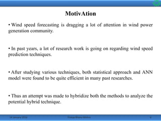
• Wind energy production from conventional energy differs in many
aspects, it is largely influenced by random wind speed change[1].
• A small change of wind speed can result in a huge change of power
output of WTG[2].
• Setting up of a wind speed measuring station is not always possible
near a wind farm[3].
• This paper reports a Weibull distribution model used to analyse past
five years of data and then uses the result of that analysis to train the
ANN.

Present Status of Wind Speed Prediction
• For maintaining the stability of the power generation in wind farms,
forecasting the wind for every small time horizon with accuracy is
essential[4].
• Wind mill setups vary in range. Some of them are:
On-shore grid connected Wind Turbine systems
Off-shore Wind turbine systems Small Wind
Hybrid Energy Decentralized systems (Floating)
• It is estimated that with the current level of technology, the ‘on-shore’
potential of wind energy can be used to harness around 65,000 MW of
electricity in India.
• Areas which can be potential sites for wind power generation in India
can be identified in the based on the following wind power density map.

• MNRE's achievement report reveals that the installed capacity of Grid
Interactive Wind Energy in India is 23444 MW as of 31st March 2015.
• The Budget of 2015 targets 60 GW of wind power in India by 2022.
• Wind power has taken a back seat in recent years and accounts for only around
1.02% of India's total installed power capacity but still holds 65.52% of total
installed renewable energy[5].
• According to the sources, the worldwide installed capacity of wind power
reached 369,553 MW where China (114,763 MW), US (65,879 MW), Germany
(39,165 MW) and Spain (22,987 MW) are ahead of India in fifth position by the
end of 2014.
• According to REN21- Global Status Report 2011 (GSR-2011), Suzlon is
among the top ten manufacturers of Wind Turbine in the world with a world
market share of 6.7%.
Contd…

MotivAtion
• Wind speed forecasting is dragging a lot of attention in wind power
generation community.
• In past years, a lot of research work is going on regarding wind speed
prediction techniques.
• After studying various techniques, both statistical approach and ANN
model were found to be quite efficient in many past researches.
• Thus an attempt was made to hybridize both the methods to analyze the
potential hybrid technique.

Objective
• The following are the main objectives of this study:
To study various methods involving wind speed prediction
To Analyse the wind energy potential of Bhubaneswar by using
Weibull model
To evaluate the reliability of Weibull model by comparing with
original wind speed data
To study Artificial Neural Network using back propagation
algorithm
To analyse the performance of a Hybrid Weibull-ANN prediction
technique

Weibull Distribution
• To establish the wind speed model by Weibull distribution usually the
probability distribution method is used.
•The Weibull distribution is widely used to describe the long-term
records of wind speed.
•The probability density function of a Weibull distribution is given by
the equation:
where, v1 = wind speed (m/s)
k = shape parameter, which affects the shape of the distribution rather than simply
shifting it.
λ = scale parameter, which stretches/shrinks the distribution curve = vm/Γ (1+1/k)
vm = monthly mean wind speed
Γ = the gamma function
where, Γ(x) = (where, u= average wind velocity)[2]

•The wind power per unit can be calculated by the following equation:
P (v1) = ½ ρ v1
3
Where, P (v1) is the power of the wind per unit area (W/m2).
ρ is the air density (kg/ m3), at sea level and at 15 °C, it is approx. 1.225 kg/m3
•If f (v1) is the Weibull density function, then the mean power density for
the Weibull function becomes:
Pw = ½ ρ v3 f(v1)
Where, Pw is the mean power density obtained by the Weibull function (W/m2).
Contd…

ANN Structure
• Originally made to mimic the biological central nervous system of
human beings, it is a large-scale parallel-distributed information
processing system which is composed of many inter-connected nonlinear
computational units (known as “neurons”).
•The network can perform many activities such as function
approximation, system identification, optimization, and adaptive control.
•The neural network based approach yields some valuable features over
traditional methods, such as adaptive learning, distributed association,
nonlinear mapping, as well as the ability to handle imprecise data.
•For predicting wind speed a neural network model can be trained by
taking a set of past measurement data .

• If there is a change in conditions, it can learn the change overtime, and
adjust itself for a more accurate prediction[6].
•So, it resembles the human brain in two respects:
Knowledge is acquired by the network from its environment through a learning
process.
Interneuron connection strengths, also known as synaptic weights, are used to
store the acquired knowledge.
•Mathematically, this process is described in the following figure:
Contd…
Where, x is the input
p is the no. of inputs.
k is the inputs received from input unit
The output of the neuron, yk, would therefore be the outcome of some
activation function on the value of vk.

• The back propagation algorithm (Rumelhart and McClelland, 1986) is
used in layered feed-forward ANNs.
• It uses supervised learning. The idea of the back propagation algorithm
is mainly to reduce this error, until the ANN learns the training data.
•The training begins with random weights, and the goal is to adjust them
so that the error will be minimal[3].
•The activation function of the artificial neurons in ANNs implementing
the back-propagation algorithm is a weighted sum (the sum of the inputs
xi multiplied by their respective weights wji) and is given by:
Contd…

Data Analysis and Histograms
• Preparing for modeling, to make the distribution of data approx. linear
normalization of data must be done, as the assumption in TS model is
that, the random noises follow Gussian distribution[7].
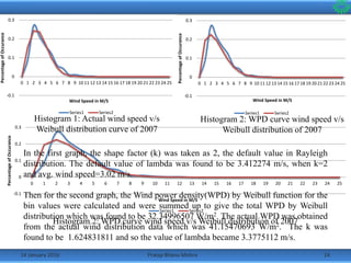
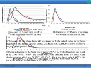
•The wind speed data was divided into linear bins from 0m/s to 25m/s
and the frequency at which they occurred on an average that year was
calculated.
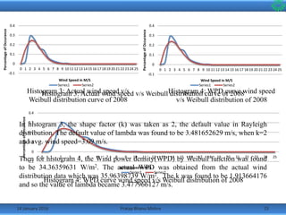
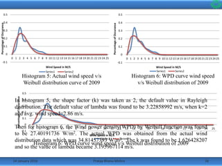
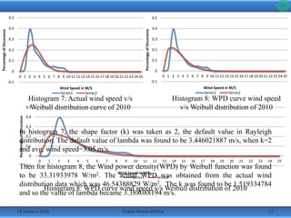
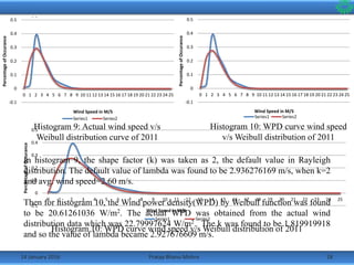
•Then taking the shape factor k=2 as per Rayleigh distribution, the
histograms along with the predicted Weibull distribution curve were
made.
•Following are the histograms of the wind data from the year 2007 to
2012.

-0.1
0
0.1
0.2
0.3
0 1 2 3 4 5 6 7 8 9 10 11 12 13 14 15 16 17 18 19 20 21 22 23 24 25
PercentageofOccurance
Wind Speed in M/S
Series1 Series2
Histogram 1: Actual wind speed v/s Weibull distribution curve of 2007
-0.1
0
0.1
0.2
0.3
0 1 2 3 4 5 6 7 8 9 10 11 12 13 14 15 16 17 18 19 20 21 22 23 24 25
Wind Speed in M/S
Series1 Series2
Histogram 2: WPD curve wind speed v/s Weibull distribution of 2007
-0.1
0
0.1
0.2
0.3
0 1 2 3 4 5 6 7 8 9 10 11 12 13 14 15 16 17 18 19 20 21 22 23 24 25
Wind Speed in M/S
Series1 Series2
-0.1
0
0.1
0.2
0.3
0 1 2 3 4 5 6 7 8 9 10 11 12 13 14 15 16 17 18 19 20 21 22 23 24 25
Wind Speed in M/S
Series1 Series2
Histogram 2: WPD curve wind speed v/s
Weibull distribution of 2007
Histogram 1: Actual wind speed v/s
Weibull distribution curve of 2007
In the first graph, the shape factor (k) was taken as 2, the default value in Rayleigh
distribution. The default value of lambda was found to be 3.412274 m/s, when k=2
and avg. wind speed=3.02 m/s.
Then for the second graph, the Wind power density(WPD) by Weibull function for the
bin values were calculated and were summed up to give the total WPD by Weibull
distribution which was found to be 32.34996507 W/m2. The actual WPD was obtained
from the actual wind distribution data which was 41.15470693 W/m2. The k was
found to be 1.624831811 and so the value of lambda became 3.3775112 m/s.

-0.1
0
0.1
0.2
0.3
0.4
0 1 2 3 4 5 6 7 8 9 10 11 12 13 14 15 16 17 18 19 20 21 22 23 24 25
Wind Speed in M/S
Series1 Series2
-0.1
0
0.1
0.2
0.3
0.4
0 1 2 3 4 5 6 7 8 9 10 11 12 13 14 15 16 17 18 19 20 21 22 23 24 25
Wind Speed in M/S
Series1 Series2
-0.1
0
0.1
0.2
0.3
0.4
0 1 2 3 4 5 6 7 8 9 10 11 12 13 14 15 16 17 18 19 20 21 22 23 24 25
Wind Speed in M/S
Series1 Series2
-0.1
0
0.1
0.2
0.3
0.4
0 1 2 3 4 5 6 7 8 9 10 11 12 13 14 15 16 17 18 19 20 21 22 23 24 25
Wind Speed in M/S
Series1 Series2
Histogram 4: WPD curve wind speed
v/s Weibull distribution of 2008
In histogram 3, the shape factor (k) was taken as 2, the default value in Rayleigh
Then for histogram 4, the Wind power density(WPD) by Weibull function was found
to be 34.36359631 W/m2. The actual WPD was obtained from the actual wind
distribution data which was 35.96398739 W/m2. The k was found to be 1.913664176
and so the value of lambda became 3.477966127 m/s.

-0.1
0
0.1
0.2
0.3
0.4
0.5
0 1 2 3 4 5 6 7 8 9 10 11 12 13 14 15 16 17 18 19 20 21 22 23 24 25
Wind Speed in M/S
Series1 Series2
-0.1
0
0.1
0.2
0.3
0.4
0.5
0 1 2 3 4 5 6 7 8 9 10 11 12 13 14 15 16 17 18 19 20 21 22 23 24 25
Wind Speed in M/S
Series1 Series2
-0.1
0
0.1
0.2
0.3
0.4
0.5
0 1 2 3 4 5 6 7 8 9 10 11 12 13 14 15 16 17 18 19 20 21 22 23 24 25
Wind Speed in M/S
Series1 Series2
-0.1
0
0.1
0.2
0.3
0.4
0.5
0 1 2 3 4 5 6 7 8 9 10 11 12 13 14 15 16 17 18 19 20 21 22 23 24 25
Wind Speed in M/S
Series1 Series2

-0.1
0
0.1
0.2
0.3
0.4
0 1 2 3 4 5 6 7 8 9 10 11 12 13 14 15 16 17 18 19 20 21 22 23 24 25
PERCENTAGEOFOCCURANCE
WIND SPEED IN M/S
Series1 Series2
-0.1
0
0.1
0.2
0.3
0.4
0 1 2 3 4 5 6 7 8 9 10 11 12 13 14 15 16 17 18 19 20 21 22 23 24 25
Wind Speed in M/S
Series1 Series2
-0.1
0
0.1
0.2
0.3
0.4
0 1 2 3 4 5 6 7 8 9 10 11 12 13 14 15 16 17 18 19 20 21 22 23 24 25
PERCENTAGEOFOCCURANCE
WIND SPEED IN M/S
Series1 Series2
-0.1
0
0.1
0.2
0.3
0.4
0 1 2 3 4 5 6 7 8 9 10 11 12 13 14 15 16 17 18 19 20 21 22 23 24 25
Wind Speed in M/S
Series1 Series2

Simulation and Evaluation of Hybrid Weibull-ANN
• The result obtained from Wind Power Density-matched Weibull
distribution was put through the time series analysis tool (ntstool) for
predicting wind speed of the three years under study more accurately.
•The input parameters to ANN model for improving the predictions are:
Frequency of sample wind speeds
%time occurrence of the wind speeds
Weibull Function of the corresponding wind speeds
Mean Power Density by Weibull of the corresponding wind speeds
Shape factor of the particular year and
Scale factor of the particular year.
•The data are randomly divided into 55% training, 20% testing and 25%
validation.

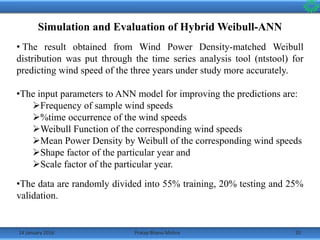
• The training data, adjust network weight according to error.
•The validation data, measures network generalization and stop training
when generalization stops improving.
•The testing data have no effect on training and provide an independent
measure of network performance during and after training.
•Calculation of Hidden Layers was done using the following equation:
where, Hn and Sn are number of hidden layer neurons and number of
data samples used in ANN model, In and On denotes number of input and
output parameters [7].
Contd…

-1.00
1.00
3.00
5.00
7.00
9.00
11.00
0 50 100 150 200 250 300 350 400
WindSpeed(m/s)
Days
2010
-1.00
0.00
1.00
2.00
3.00
4.00
5.00
6.00
7.00
8.00
9.00
0 100 200 300 400
WindSpeed(m/s)
Days
2011
0.00
1.00
2.00
3.00
4.00
5.00
6.00
7.00
8.00
9.00
0 100 200 300 400
WindSpeed(m/s)
Days
2012
Contd…

Contd…
• For training of ANN model 101 data points were taken from the
average daily wind speed curve of Bhubaneswar for the year 2010, 2011
and 2012.
•The sensitivity test was performed to validate the number of hidden
layer neurons by changing the no. of hidden layers by ±1 from hidden
layer neurons calculated by the previously given equation.
•The multilayer perceptron (MLP) neural network architecture (6-13-1)
with best validation performance was used to analyse the accuracy of
prediction of wind speed by the proposed hybrid model.
•The results were analysed using:
Performance Plot
Regression Plot
Input-Error Cross-Correlation Plot

•The performance plots of ANN model demonstrates that mean square
error becomes minimum as number of epochs increases. The epoch is
one complete sweep of training, testing and validation.
Contd…
Performance Plot for 2010Performance Plot for 2011Performance Plot for 2012

• The correlation coefficient (R-value) shows the association among
outputs and target value of ANN model. R value of 1and 0 measures a
strong, random association respectively.
Regression Plot for 2011
Contd…

• The Input-Error cross-correlation plot shows how the networks error
at any given time is correlated with networks input at different time lags.
Contd…
Input-Error Cross-Correlation Plot for 2010

conclusion
• The data collected was matched with the Weibull distribution in the
context of both wind power density and wind speed distribution for
accuracy purpose.
•Then an ANN model was developed with Time-series tool (ntstool) for
improving wind speed curves created by Weibull distribution.
•The correlation coefficient (R-value) of 0.99992 and slope 1 was
achieved forboth 2010 and 2011 while anR-value of 0.99994and slope
1was achieved for 2012 for the whole data set, showing high prediction
accuracy of the developed ANN Model.
•Data analysis confirms that the Weibull distribution is an adequate
technique for describing the daily average wind speed distribution. But
using a Hybrid ANN method gives superior result and can help in more
accurate forecasting.

Future scope
• In future the equations of Weibull distribution can be merged with
other non-linear equations for handling nonlinearity and stochastic
uncertainty problems associated with wind speed data and then
hybridising it with ANN will be more effective.
•Addition of any GUI which helps in predicting future data with
MATLAB will be helpful for validating the results as well as finding the
MAPE.
•Also wind data of a windier region will give better forecasting results.

References
[1] Wang Ruigang, Wenyi Li, and B. Bagen. "Development of Wind Speed
Forecasting Model Based on the Weibull Probability Distribution", 2011
International Conference on Computer Distributed Control and Intelligent
Environmental Monitoring, 2011.
[2] Yuehua, Liu, Jiang Yingni, and Gong Qingge. "Analysis of wind energy
potential using the Weibull model at Zhurihe", 2011 International
Conference on Consumer Electronics Communications and Networks
(CECNet), 2011.
[3] Liang Wu. "A study on wind speed prediction using artificial neural network
at Jeju Island in Korea-I", 2009 Transmission & Distribution Conference &
Exposition Asia and Pacific, 10/2009.
[4] M. Negnevitsky, P. Mandal, A. K. Srivastava, "An overview of forecasting
problems and techniques in power systems," Power & Energy Society
General Meeting, 2009. PES '09. IEEE, vol., no., pp.1-4, 26-30 July 2009.

[5] http://www.indianwindpower.com/
[6] Xiao-Hua Yu. "Applications of Neural Networks to Dynamical System
Identification and Adaptive Control", Studies in Computational Intelligence,
2008.
[7] P. Ramasamy, S.S. Chandel, Amit Kumar Yadav. "Wind speed prediction in
the mountainous region of India using an artificial neural network model",
Renewable Energy, Volume 80, August 2015, Pages 338–347.
Contd…

Publications
• Pratap Bhanu Mishra, Dr. S.M Ali. “Advances in Wind Energy”, 2014
All India Seminar on Modern Trends in Power System Operation,
Control & Management, Instiute of Engineers, pp. 158-163.
• Mrs. Lipika Nanda, P.B Mishra. “Analysis of Wind Speed Prediction
Techinque by hybrid Weibull-ANN Model”, 2015 IEEE Power,
Communication and Information Technology Conference (PCITC)
Siksha ‘O’Anusandhan University, Bhubaneswar, India.

Presentation1

More Related Content

What's hot

Similar to Presentation1

Presentation1