Return Decomposition By Long Chen and Xinlei Zhao Presentation by Michael-Paul James Directly modeling discount rate news and backing out cash flow news adds residual news to the latter ○ The method has led to erroneous conclusions: ■ Larger relative DR variance ■ Value stocks earn higher returns due to higher βCF ■ βCF is more important than total βtotal ○ DR news cannot be accurately estimated (low predictive power) and backed out CF news inherits large misspecification error of DR ○ Modeled Treasury bonds reveals higher CF variance with no real CF risk ○ Minor changes in predictive variables produce opposite results Directly modeling cash flow news, discount rate news, and residual ○ Value firms have both lower modeled CF betas and DR betas, but higher residual betas, indicating that the results in the current literature are driven by the residual news.

1. Return Decomposition
By Long Chen and Xinlei Zhao
Presentation by Michael-Paul James
1

2. Table of contents
2
Introduction
story, questions, context, issues,
literature
01
Theory
Theoretical Discussion
Decomposition procedure
An ICAPM interpretation
Implications
Current literature
02
Treasury
Treasury Bond Returns
03
Equity
Equity Returns
Variances of the market portfolio
Cross-sectional patterns
The benchmark case.
Replacing with similar variables.
04
Remedies
Direct modeling of the CF news
Dividend growth rate; ROE;
Bayesian model averaging approach
Principal component analysis
Some motivated choices
Summary of results
05
Robustness
Further Robustness Checks
Industry portfolios
Post-1952 data
Other robustness checks
06
Conclusions
07
Michael-Paul James

3. Introduction
01
story, questions, context, issues, literature
3
Michael-Paul James

4. History of News Decomposition
4
● Return beta decomposed into discount rate and cash flow news to
measure time-series and cross sectional variations (Campbell and
Shiller, 1988)
○ Cash flow (CF) news captures firm fundamentals
○ Discount rate (DR) news captures risk aversion and sentiment
● Return decomposition approach
○ For simplicity, researchers directly modeled discount rate news
then labeled the residual as cash flow news.
○ Issues
■ Captures misspecification error of discount rate news, which is
inherently difficult to measure.
■ Omitted DR variables are passed to CF, distorting relationship
Michael-Paul James

5. Seeking Misspecification Confirmation
5
● Return decomposition approach on Treasury bond returns
○ Variation should be driven solely by discount rate news
■ Fixed cash flows (βCF
= 0): no nominal cash flow uncertainty
■ Real interest rate and inflation shocks solely effect returns
■ Any cash flow news would be the aggregation of modeling
noise
○ Estimated variance of CF news is greater than or equal to DR news
■ Longer maturity bonds had even higher βCF
■ Likely caused by missing state variables in DR news
Michael-Paul James

6. Equities and Noise
6
● Playing with the variables
○ Benchmark case:
■ 10-year smoothed price-earnings (PE) ratio
■ Term spread (long-term less short-term bond yields)
■ Value spread (log book-to-market small value less small
growth stocks)
○ Persistence drives impact of state variables, leading to estimation
reversals with close substitutes and differing sample periods
○ Substitutes for 10-year smoothed price-earnings (PE) ratio
■ 1-year PE ratio ■ Dividend yield
■ Book-to-market ratio ■ Book-to-market spread
Michael-Paul James

7. Substitutes and Reversals
7
● Benchmark case concludes DR variance is greater than CF variance
○ Driven by high persistence of state variables
● Substitutes effects
○ Improved explanatory power (>R2
) and greater significance of
other variables
○ Lower value stock βCF
, generally smaller than βDR
● Substitutes for 10-year smoothed price-earnings (PE) ratio
○ 1-year PE ratio: CF variance is greater than or equal to DR
○ Book-to-market ratio: CF variance is greater than or equal to DR
○ Dividend yield: CF variance slightly higher than DR
○ Book-to-market spread: CF variance is greater than DR
Michael-Paul James

8. Not Robustness, Specification
8
● Model misspecification leads to opposite conclusions: not a robustness
issue but a crucial one
● Predictive variables relate to the macroeconomy therefore all are well
motivated, but not necessarily correct.
● Analysis must directly measure or model CF and DR news individually
to allow for a third residual term (error) to maintain a balanced
relationship between variables
● Model uncertainty can be leveraged with the Bayesian model
averaging approach to a large set of predictive variables
Michael-Paul James

9. Theory
02
Theoretical Discussion
Decomposition procedure
An ICAPM interpretation
Implications
Current literature
9
Michael-Paul James

10. Decomposition Procedure
10
● Decomposition of unexpected returns
● rt+1
equity return ● Et
expectation operator
● ρ constant marginally less than 1 ● Δdt
dividend growth rate
● et+1
unexpected market return ● eCF,t+1
cash flow news
● -eDR,t+1
discount rate news
Michael-Paul James

11. Decomposition Procedure
11
● Market beta
Michael-Paul James

12. Decomposition Procedure
12
● Vector of state variables (first order vector autoregression, VAR)
● Discount rate news
Michael-Paul James

13. Decomposition Procedure
13
● CF news as difference between total unexpected return and DR news
● Adjustments
○ Excess returns in VAR and beta calculation
○ Lag of market news (mitigates stale-price problem)
Michael-Paul James

14. ICAPM Interpretation
14
● Approximate discrete-time version of Merton’s intertemporal CAPM
● ri,t+1
return for asset i ● rf,t+1
risk-free rate
● σ2
M
market portfolio variance ● γ risk-aversion coefficient (>1)
● Integrate VAR system: state variables combined into either CF or DR
Michael-Paul James

15. Implications
15
● VAR system (assumed)
● cov(ei,t
,u2,t
)=0, xt
is predictable only by its lag variables. u1,t+1
& u2,t+1
are
innovations in the return and x
Michael-Paul James

16. Omitting the Second State Variable x
16
● Omitted variable ● shock → yt
= u1,t
+ α2
xt-1
● Both betas change in opposite directions when α1
> 0
● Simultaneous impact on both betas exaggerate/inverse relationship
Michael-Paul James

17. Conclusion
17
● “The essence of the residual based return decomposition approach is
to compare the modeled part with the residual; conclusions are
usually a choice between more important and less important or
between higher and lower.”
● “Since model misspecification can lead to opposite conclusion this
sensitivity is not a robustness issue; it is a vital issue.”
Michael-Paul James

18. Treasury
03
Treasury Bond Returns
18
Michael-Paul James

19. Setting up the Treasury Regression
19
● Log linear approximation
● Discount rate news
● Zero coupon bonds (Campbell & Ammer, 1993): CF news equals zero
Michael-Paul James

20. Table
1:
Variance
&
beta
decomposition
of
Treasury
bond
excess
returns
20
Table 1: Variance and beta decomposition of Treasury bond excess returns
Panel A: Variance decomposition
Variables in VAR Variances (%)
Term spread Real rate Inflation
Credit
spread Var (CF) Var (DR) Cov(CF, DR)
∎ 0.33 0.17 0.09
∎ 0.53 0.08 0.14
∎ ∎ 0.42 0.18 0.16
∎ ∎ 0.18 0.18 0.03
∎ ∎ ∎ 0.21 0.16 0.06
∎ ∎ ∎ 0.17 0.16 0.02
∎ ∎ ∎ ∎ 0.19 0.13 0.03
Panel B: Beta decomposition using Ibbotson data
Full Sample
βCF
βDR
βCF
−βDR
S.E.
30-day T-Bill (1) 0.14 0.02 0.12 -0.06
Long-term bond (2) 1.02 0.51 0.51 -0.46
(2) – (1) 0.88 0.49
S.E. of (2) – (1) -0.27 -0.26
Excess returns
16% < R2
< 35%
Highest with 4 variables
Var(CF) ≥ Var(DR)
Var(CF) ≡ 0
Var(CF) =
unspecified Var(DR)
>
>
>
=
>
>
>
>
>
>
Long-term bond has
higher and
faster-growing βCF
, not
0 as expected
Michael-Paul James

21. Table
1:
Variance
&
beta
decomposition
of
Treasury
bond
excess
returns
21
We apply the return decomposition approach to Treasury bond returns using annual data (aggregated from monthly data) covering 1953–2002.
In Panel A, we decompose the excess return of intermediate-term Treasury bond into discount rate (DR) news and cash flow (CF) news. We
then report the variances of the two components and their covariance. The state variables include different combinations of the term spread
(the difference between the long-term and short-term bond yields), real interest rate, inflation, and credit spread (Baa over Aaa bond yield). The
plus signs indicate the selected variables in each scenario. In Panel B, we use the intermediate-term Treasury bond (from Panel A) as our bond
market portfolio and calculate the discount rate beta and cash flow beta for 30-day T-bill and long-term bond. Similarly, in Panel C1, we
calculate the betas for Fama-Bliss zero-coupon bonds ranging from two to five years. In Panel C2, we calculate the betas for the Fama bond
portfolios ranging from one year to 10 years. In Panels B and C, the “Diff” columns report the differences in betas of two adjacent portfolios with
different maturities; the “βCF − βDR” columns report the differences in cash flow and discount rate betas of the same portfolio. In Panels B and
C, we report bootstrap standard errors (S.E.) from 10,000 simulated realizations.
Table 1: Variance and beta decomposition of Treasury bond excess returns
Maturity βCF
Diff. S.E. of Diff βDR
Diff. S.E. of Diff βCF
−βDR
S.E.
Panel C1: Fama-Bliss zero coupon bonds
2-year 0.18 0.11 0.07 -0.12
3-year 0.31 0.13 -0.06 0.24 0.12 -0.06 0.08 -0.23
4-year 0.42 0.11 -0.05 0.31 0.08 -0.05 0.11 -0.31
5-year 0.52 0.1 -0.05 0.38 0.07 -0.05 0.14 -0.38
Panel C2: Fama bond portfolios
1-year 0.25 0.1 0.15 -0.14
2-year 0.4 0.14 -0.06 0.21 0.11 -0.04 0.19 -0.19
3-year 0.53 0.13 -0.05 0.32 0.1 -0.05 0.21 -0.25
4-year 0.61 0.08 -0.05 0.39 0.08 -0.05 0.21 -0.29
5-year 0.71 0.1 -0.08 0.36 −0.03 -0.07 0.35 -0.33
10-year 0.73 0.02 -0.07 0.45 0.09 -0.07 0.28 -0.36
Long-term bond has
higher βCF
, not 0 as
expected
>
>
>
>
>
>
>
>
>
>
False model:
Treasury bonds have
no nominal CF risk
Unrealistic: CF risk is
greater than the DR risk

22. Equity
04
Equity Returns
Variances of the market portfolio
Cross-sectional patterns
The benchmark case.
Replacing the benchmark case with similar variables.
22
Michael-Paul James

23. Table
2:
Variance
decomposition
of
the
equity
market
portfolio
23
Table 2: Variance decomposition of the equity market portfolio
Models 1 2 3 4 5 6 7 8
Excess return ∎ ∎ ∎ ∎ ∎ ∎ ∎ ∎
Term spread ∎ ∎ ∎ ∎ ∎ ∎ ∎ ∎
10-year PE ratio ∎
Value spread ∎ ∎ ∎ ∎ ∎ ∎ ∎ ∎
1-year PE ratio ∎ ∎
Dividend yield ∎
Book-to-market ratio ∎ ∎
BM spread ∎ ∎
Stock variance ∎
Corporate issue ∎ ∎
Panel A: Monthly data (1929–2001)
Variance of CF (%) 0.06 0.44 0.05 0.14 0.10 0.36 0.57 0.05
Variance of DR (%) 0.27 0.05 0.23 0.11 0.21 0.10 0.30 0.27
Cov(CF, DR ) (%) −0.01 −0.09 0.01 0.02 −0.01 −0.08 −0.28 −0.011
Panel B: Monthly data (1952–2001)
Variance of CF (%) 0.04 0.21 0.06 0.04 0.11 0.20 0.21 0.06
Variance of DR (%) 0.09 0.02 0.06 0.11 0.04 0.02 0.06 0.05
Cov(CF, DR ) (%) 0.02 −0.03 0.03 0.02 0.02 −0.02 −0.05 0.03
Panel C: Annual data (1929–2001)
Variance of CF (%) 0.42 5.00 0.40 2.91 1.20 5.95 3.04 0.55
Variance of DR (%) 3.21 0.36 2.79 1.59 1.94 1.05 0.9 2.16
Cov(CF, DR ) (%) −0.14 −0.78 0.14 −0.44 0.14 −1.86 −0.60 0.13
Panel D: Annual data (1952–2001)
Variance of CF (%) 0.33 2.30 0.55 0.48 1.29 2.64 2.5 0.67
Variance of DR (%) 1.32 0.17 0.92 2.03 0.50 0.28 0.5 0.79
Cov(CF, DR ) (%) 0.46 0.07 0.57 −0.02 0.42 −0.16 −0.23 0.56
Relative important of
CF & DR variance is
sensitive to changes of
state variables
Column 1.A: DR > CF,
Campbell consistent,
Drop P/E: (2.A) CF>DR
P/E dominates due to
persistence
10 year P/E (not
stationary) hasn’t clear
reason for superiority
to 1-year P/E, dividend
yield, book-to-market
Michael-Paul James

24. Table 3: CAPM beta, cash flow beta, and discount rate beta
Panel A: CAPM beta, cash flow beta, and discount rate beta
Before 1963:6 After 1963:7
βCAPM
Growth 2 3 4 Value Growth 2 3 4 Value
Small 1.73 1.65 1.54 1.46 1.56 1.43 1.22 1.08 1.00 1.01
2 1.15 1.28 1.26 1.34 1.50 1.42 1.16 1.03 0.97 1.04
3 1.21 1.14 1.21 1.24 1.56 1.36 1.10 0.97 0.89 0.97
4 0.97 1.10 1.14 1.30 1.67 1.25 1.07 0.96 0.89 0.97
Large 0.95 1.92 1.04 1.29 1.48 1.00 0.94 0.84 0.77 0.77
βCF
Small 0.58 0.51 0.43 0.46 0.55 0.05 0.06 0.08 0.09 0.13
2 0.30 0.36 0.39 0.41 0.49 0.03 0.08 0.10 0.11 0.12
3 0.32 0.29 0.32 0.37 0.51 0.03 0.09 0.10 0.12 0.12
4 0.20 0.27 0.32 0.37 0.53 0.02 0.09 0.11 0.11 0.13
Large 0.20 0.19 0.29 0.34 0.42 0.02 0.08 0.08 0.11 0.11
βDR
Small 1.37 1.63 1.41 1.37 1.39 1.63 1.35 1.17 1.11 1.11
2 1.04 1.20 1.16 1.20 1.30 1.51 1.20 1.05 0.94 1.01
3 1.16 1.02 1.09 1.08 1.32 1.39 1.08 0.94 0.82 0.93
4 0.86 0.99 1.00 1.10 1.41 1.25 1.03 0.87 0.78 0.86
Large 0.87 0.82 0.89 1.07 1.19 1.00 0.86 0.73 0.63 0.67
Table
3:
CAPM
beta,
cash
flow
beta,
and
discount
rate
beta
24
We use the same dataset as in
Campbell and Vuolteenaho (2004a).
Panel A reports, for both the pre-1963
and post-1963 periods, the CAPM betas,
cash flow betas, and discount rate betas
of the 25 portfolios sorted by size and
market-to-book ratio. The same state
variables in Campbell and Vuolteenaho
(2004a) are used to obtain the cash flow
betas and discount rate betas. In Panel
B, average returns of portfolios,
including the 25 Fama-French portfolios
and 20 additional portfolios as in
Campbell and Vuolteenaho (2004a), are
first obtained and then regressed
cross-sectionally on the betas.
Panel B: The cross-section of equity returns
CAPM Intercept β Adj. R2 Intercept β Adj. R2
Coeff. 0.26% 0.54% 40.13% 0.80% −0.18% 2.10%
S.E. (0.13%) (0.10%) (0.14%) (0.13%)
Two Beta ICAPM Intercept βCF
βDR
Adj. R2
Intercept βCF
βDR
Adj. R2
Coeff. 0.42% 1.24% 0.10% 44.76% 0.07% 5.30% 0.10% 49.99%
S.E. (0.15%) (0.66%) (0.31%) (0.13%) (0.80%) (0.08%)
CF betas carry
variation from growth to
value; DR betas carry
small to large
Campbell and
Voulteenaho dataset
replication, 25 FF sort +
20, 1929-2001
CAPM explains ~2%
ICAPM explains ~50%
Michael-Paul James

25. Table
4:
Betas
with
a
subset
of
or
similar
state
variables
as
in
Campbell
and
Vuolteenaho
(2004a)
25
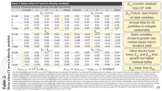
Table 4: Betas with a subset of or similar state variables as in Campbell and Vuolteenaho
Panel A: VAR variables include the excess equity market return, term spread, and value spread
Panel A1: Betas
βCF
Growth 2 3 4 Value Diff
Small 1.74 1.51 1.39 1.35 1.44 −0.30 [0.07]
2 1.63 1.45 1.34 1.25 1.35 −0.28 [0.07]
3 1.54 1.36 1.23 1.15 1.26 −0.28 [0.07]
4 1.37 1.29 1.17 1.07 1.20 −0.17 [0.07]
Large 1.09 1.09 0.95 0.91 0.97 −0.12 [0.06]
Diff −0.65 −0.42 −0.44 −0.44 −0.47
[0.10] [0.09] [0.08] [0.07] [0.07]
βDR
Growth 2 3 4 Value Diff
Small −0.03 −0.07 −0.12 −0.13 −0.18 0.15 [0.03]
2 −0.05 −0.14 −0.16 −0.17 −0.19 0.14 [0.03]
3 −0.08 −0.15 −0.16 −0.19 −0.19 0.11 [0.03]
4 −0.06 −0.15 −0.16 −0.15 −0.19 0.13 [0.03]
Large −0.05 −0.12 −0.11 −0.15 −0.17 0.12 [0.03]
Diff 0.02 0.05 −0.01 0.02 0.01
[0.05] [0.04] [0.04] [0.03] [0.03]
Panel A2: Cross-sectional regression
Intercept βCF βDR Adj. R2
Coeff. −0.04% 0.16% −3.65% 52.36%
S.E. (0.14%) (0.08%) (0.51%)
Excluded PE ratio,
-increases CF value, -
σ2
CF
> σ2
DR
-Inverts growth to value
-R2
improves bench
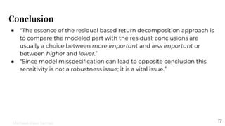
Campbell and Vuolteenaho (2004a) use four state
variables in their VAR system: excess equity market
return, term spread, 10-year smoothed PE ratio, and
the value spread. In Panel A, the 10-year PE ratio is
excluded; we report discount rate and cash flow
betas, as well as cross-sectional regression
coefficients. In Panels B1–B4, we report the cash flow
betas when the 10-year PE ratio is replaced, in
sequence, by (i) 1-year PE ratio, (ii) dividend yield, (iii)
book-to-market ratio, and (iv) the book-to-market
spread plus the corporate issue. The standard errors
of the differences in the betas between large and
small, as well as value and growth firms are obtained
through bootstrapping 10,000 realizations. This table
only reports results during 1963:07–2001:12.
Michael-Paul James

26. Table
4:
Betas
with
a
subset
of
or
similar
state
variables
as
in
Campbell
and
Vuolteenaho
(2004a)
26
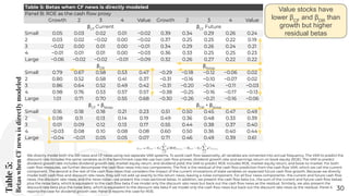
Campbell and Vuolteenaho (2004a) use four state
variables in their VAR system: excess equity market
return, term spread, 10-year smoothed PE ratio, and
the value spread. In Panel A, the 10-year PE ratio is
excluded; we report discount rate and cash flow
betas, as well as cross-sectional regression
coefficients. In Panels B1–B4, we report the cash flow
betas when the 10-year PE ratio is replaced, in
sequence, by (i) 1-year PE ratio, (ii) dividend yield, (iii)
book-to-market ratio, and (iv) the book-to-market
spread plus the corporate issue. The standard errors
of the differences in the betas between large and
small, as well as value and growth firms are obtained
through bootstrapping 10,000 realizations. This table
only reports results during 1963:07–2001:12.
Table 4: Betas with a subset of or similar state variables as in Campbell and Vuolteenaho
Panel B1: VAR variables include the excess equity market return, term spread, log 1-year PE ratio,
and value spread
βCF
Growth 2 3 4 Value Diff
Small 0.33 0.27 0.24 0.23 0.24 −0.09 [0.02]
2 0.28 0.24 0.21 0.19 0.20 −0.08 [0.03]
3 0.24 0.21 0.20 0.17 0.19 −0.05 [0.03]
4 0.22 0.21 0.19 0.16 0.18 −0.04 [0.03]
Large 0.15 0.17 0.14 0.14 0.14 −0.01 [0.02]
Diff −0.18 −0.10 −0.10 −0.09 −0.10
[0.04] [0.03] [0.03] [0.03] [0.03]
Panel B2: VAR variables include the excess equity market return, term spread, dividend yield, and
value spread
Small 0.98 0.87 0.81 0.80 0.87 −0.11 [0.04]
2 0.91 0.84 0.80 0.76 0.83 −0.08 [0.04]
3 0.87 0.81 0.74 0.71 0.77 −0.10 [0.04]
4 0.77 0.77 0.71 0.66 0.74 −0.03 [0.04]
Large 0.63 0.66 0.58 0.58 0.61 −0.02 [0.04]
Diff −0.35 −0.21 −0.23 −0.22 −0.26
[0.06] [0.05] [0.04] [0.04] [0.04]
Panel B3: VAR variables include the excess equity market return, term spread, book-to-market
ratio, and value spread
Small 0.72 0.59 0.52 0.52 0.55 −0.17 [0.04]
2 0.63 0.54 0.50 0.48 0.52 −0.11 [0.04]
3 0.59 0.51 0.46 0.44 0.47 −0.12 [0.04]
4 0.53 0.48 0.44 0.39 0.43 −0.10 [0.04]
Large 0.42 0.42 0.36 0.35 0.36 −0.06 [0.03]
Diff −0.30 −0.17 −0.16 −0.17 −0.19
[0.05] [0.05] [0.04] [0.04] [0.04]
10-yr P/E replacement
All CF declines V to G
Log 1-year P/E
Dividend yield
Book-to-market

27. Table
4:
Betas
with
a
subset
of
or
similar
state
variables
as
in
Campbell
and
Vuolteenaho
(2004a)
27
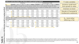
Table 4: Betas with a subset of or similar state variables as in Campbell and Vuolteenaho
Panel B4: VAR variables include the excess equity market return, term spread, book-to-market
spread, corporate issue, and value spread
Small 0.64 0.52 0.46 0.47 0.50 −0.14 [0.08]
2 0.55 0.48 0.45 0.43 0.48 −0.07 [0.08]
3 0.53 0.47 0.41 0.39 0.44 −0.09 [0.08]
4 0.46 0.44 0.40 0.34 0.39 −0.07 [0.08]
Large 0.38 0.39 0.33 0.31 0.33 −0.05 [0.07]
Diff −0.26 −0.13 −0.13 −0.16 −0.17
[0.11] [0.10] [0.09] [0.08] [0.08]
Panel B5: VAR variables include the excess equity market return, term spread, updated 10-year
smoothed PE ratio, and value spread
Small 0.34 0.27 0.24 0.23 0.25 −0.09 [0.03]
2 0.29 0.24 0.22 0.19 0.21 −0.08 [0.03]
3 0.25 0.22 0.20 0.20 0.17 −0.08 [0.03]
4 0.23 0.21 0.19 0.16 0.18 −0.05 [0.03]
Large 0.16 0.17 0.15 0.14 0.14 −0.02 [0.02]
Diff −0.18 −0.10 −0.09 −0.09 −0.11
[0.04] [0.03] [0.03] [0.03] [0.03]
BM + corp issue + value
spread
Updated 10-year
smoothed PE ratio (lag)
Campbell and Vuolteenaho (2004a) use four state
variables in their VAR system: excess equity market
return, term spread, 10-year smoothed PE ratio, and
the value spread. In Panel A, the 10-year PE ratio is
excluded; we report discount rate and cash flow
betas, as well as cross-sectional regression
coefficients. In Panels B1–B4, we report the cash flow
betas when the 10-year PE ratio is replaced, in
sequence, by (i) 1-year PE ratio, (ii) dividend yield, (iii)
book-to-market ratio, and (iv) the book-to-market
spread plus the corporate issue. The standard errors
of the differences in the betas between large and
small, as well as value and growth firms are obtained
through bootstrapping 10,000 realizations. This table
only reports results during 1963:07–2001:12.
R2
drops: 50% to 12%
Michael-Paul James

28. Remedies
05
Some Potential Remedies
Dividend growth rate
Bayesian model averaging approach
Some motivated choices
28
Direct modeling of the CF news
Return on equity
Principal component analysis
Summary of results
Michael-Paul James

29. Table
5:
Betas
when
CF
news
is
directly
modeled
29
We directly model both the DR news and CF news using two separate VAR systems. To avoid cash flow seasonality, all variables are converted into annual frequency. The VAR to predict the
discount rate includes the same variables as in the benchmark case.We use two cash flow proxies: dividend growth rate and earnings return on book equity (ROE). The VAR to predict
dividend growth rate includes dividend growth rate, market equity return, and dividend yield; the VAR to predict ROE includes ROE, market equity return, and book-to-market. For both
cash flow measures, we further decompose the cash flow news into two components. The first is the residual of the cash flow prediction from the cash flow VAR, which we call the current
component. The second is the rest of the cash flow news that considers the impact of the current innovations of state variables on expected future cash flow growth. Because we directly
model both cash flow and discount rate news, they will not add up exactly to the return news, leaving a noise component. For all four news components– the current and future cash flow
news, the discount rate news, and the news noise—we present the cross-sectional betas. In addition, we present the cash flow beta (i.e., the sum of the current and future cash flow betas)
plus the noise beta, which is equivalent to the cash flow beta if we model only the discount rate news but back out the cash flow news as the residual. Similarly, we also present the
discount rate beta plus the noise beta, which is equivalent to the discount rate beta if we model only the cash flow news but back out the discount rate news as the residual. Panel A
reports the case for dividend growth rate; Panel B reports the case for ROE.
Table 5: Betas when CF news is directly modeled
Panel A: Dividend growth rate as the cash flow proxy
Growth 2 3 4 Value Growth 2 3 4 Value
βCF
Current βCF
Future
Small 0.54 0.35 0.27 0.21 0.29 0.51 0.43 0.38 0.35 0.37
2 0.42 0.32 0.23 0.26 0.26 0.48 0.35 0.36 0.32 0.31
3 0.35 0.25 0.21 0.24 0.19 0.47 0.39 0.34 0.33 0.30
4 0.21 0.20 0.18 0.18 0.26 0.45 0.41 0.31 0.32 0.35
Large 0.10 0.18 0.14 0.17 0.12 0.44 0.36 0.36 0.31 0.37
βDR
βNoise
Small 0.84 0.69 0.59 0.55 0.45 −0.94 −0.63 −0.47 −0.36 −0.43
2 0.80 0.52 0.56 0.40 0.36 −0.88 −0.58 −0.48 −0.45 −0.39
3 0.82 0.62 0.50 0.48 0.41 −0.88 −0.57 −0.45 −0.45 −0.33
4 0.97 0.74 0.52 0.58 0.55 −0.75 −0.57 −0.41 −0.43 −0.55
Large 0.99 0.69 0.66 0.54 0.61 −0.65 −0.59 −0.50 −0.45 −0.45
βCF
+ βNoise
βDR
+ βNoise
Small 0.10 0.16 0.17 0.20 0.23 −0.11 0.06 0.11 0.18 0.02
2 0.02 0.09 0.11 0.14 0.18 −0.07 −0.06 0.08 −0.05 −0.04
3 −0.06 0.07 0.10 0.12 0.16 −0.05 0.05 0.05 0.02 0.08
4 −0.09 0.04 0.09 0.06 0.06 0.22 0.17 0.11 0.16 −0.00
Large −0.11 −0.06 0.00 0.02 0.05 0.34 0.10 0.16 0.08 0.16
Annual data for 25
portfolios to mitigate
seasonality
State variables:
dividend growth rate,
market equity return,
dividend yield
Value stocks have
lower βCF
and βDR
than
growth but higher
residual betas
βCF
lower than βDR
βCF
Current: residual
from CF VAR
βCF
Future: plus impact
of state variables

30. Table
5:
Betas
when
CF
news
is
directly
modeled
30
We directly model both the DR news and CF news using two separate VAR systems. To avoid cash flow seasonality, all variables are converted into annual frequency. The VAR to predict the
discount rate includes the same variables as in the benchmark case.We use two cash flow proxies: dividend growth rate and earnings return on book equity (ROE). The VAR to predict
dividend growth rate includes dividend growth rate, market equity return, and dividend yield; the VAR to predict ROE includes ROE, market equity return, and book-to-market. For both
cash flow measures, we further decompose the cash flow news into two components. The first is the residual of the cash flow prediction from the cash flow VAR, which we call the current
component. The second is the rest of the cash flow news that considers the impact of the current innovations of state variables on expected future cash flow growth. Because we directly
model both cash flow and discount rate news, they will not add up exactly to the return news, leaving a noise component. For all four news components– the current and future cash flow
news, the discount rate news, and the news noise—we present the cross-sectional betas. In addition, we present the cash flow beta (i.e., the sum of the current and future cash flow betas)
plus the noise beta, which is equivalent to the cash flow beta if we model only the discount rate news but back out the cash flow news as the residual. Similarly, we also present the
discount rate beta plus the noise beta, which is equivalent to the discount rate beta if we model only the cash flow news but back out the discount rate news as the residual. Panel A
reports the case for dividend growth rate; Panel B reports the case for ROE.
Table 5: Betas when CF news is directly modeled
Panel B: ROE as the cash flow proxy
Growth 2 3 4 Value Growth 2 3 4 Value
βCF
Current βCF
Future
Small 0.05 0.03 0.02 0.01 −0.02 0.39 0.34 0.29 0.26 0.24
2 0.03 0.02 −0.02 0.00 −0.02 0.37 0.25 0.25 0.22 0.19
3 −0.02 0.00 0.01 0.00 −0.01 0.34 0.29 0.26 0.24 0.21
4 −0.01 0.01 0.01 0.00 −0.03 0.36 0.33 0.25 0.25 0.23
Large −0.06 −0.02 −0.02 −0.01 −0.09 0.32 0.26 0.27 0.22 0.22
βDR
βNoise
Small 0.79 0.67 0.58 0.53 0.47 −0.29 −0.18 −0.12 −0.06 0.02
2 0.80 0.52 0.58 0.41 0.37 −0.31 −0.16 −0.10 −0.07 0.02
3 0.86 0.64 0.52 0.49 0.42 −0.31 −0.20 −0.14 −0.11 −0.03
4 0.98 0.76 0.53 0.57 0.57 −0.38 −0.25 −0.16 −0.17 −0.13
Large 1.01 0.71 0.70 0.55 0.68 −0.30 −0.26 −0.21 −0.16 −0.06
βCF
+ βNoise
βDR
+ βNoise
Small 0.16 0.18 0.18 0.21 0.23 0.51 0.50 0.45 0.47 0.49
2 0.08 0.11 0.13 0.14 0.19 0.49 0.36 0.48 0.33 0.39
3 0.01 0.09 0.12 0.13 0.17 0.55 0.44 0.38 0.37 0.40
4 −0.03 0.08 0.10 0.08 0.08 0.60 0.50 0.36 0.40 0.44
Large −0.04 −0.01 0.05 0.05 0.07 0.71 0.46 0.49 0.39 0.61
Value stocks have
lower βCF
and βDR
than
growth but higher
residual betas

31. Table
6:
Cash
flow
betas
with
Bayesian
model
averaging
method
31
We apply the Bayesian model averaging method, following Avramov (2002) and Cremers (2002), to a large set of predictive variables. In particular, we assign equal prior probability to each
combination of state variables, but update the posterior probability according to the predictability of market excess returns. We then report the expected cash flow betas of 25 size and
book-to-market portfolios using the posterior probability. The first three panels vary only because we replace the 10-year PE ratio by either the 1-year PE ratio or the dividend yield. In Panel
D, we replace the value spread by the book-to-market spread and the market-to-book spread, following Liu and Zhang (2008).
Table 6: Cash flow betas with Bayesian model averaging method
Avramov Cremers (φ = 3.25)
βCF
Growth 2 3 4 Value Growth 2 3 4 Value
Panel A: VAR variables include the excess equity market return, term spread, 10-year PE ratio,
value spread, credit spread, long-term corporate bond return, book-to-market ratio, 3-month T-bill
rate, inflation, corporate issuing activity, and stock variance.
Small 0.41 0.39 0.41 0.41 0.45 0.51 0.47 0.46 0.46 0.49
2 0.39 0.41 0.42 0.44 0.46 0.47 0.47 0.47 0.47 0.49
3 0.40 0.42 0.41 0.42 0.44 0.47 0.47 0.45 0.44 0.47
4 0.37 0.41 0.41 0.40 0.44 0.44 0.45 0.44 0.42 0.46
Large 0.30 0.36 0.32 0.34 0.36 0.35 0.39 0.34 0.35 0.36
Panel B: VAR variables are the same as in Panel A except that the 10-year PE ratio is replaced by
the 1-year PE ratio.
Small 0.55 0.50 0.49 0.48 0.51 0.62 0.54 0.52 0.51 0.54
2 0.52 0.50 0.49 0.49 0.51 0.57 0.54 0.51 0.51 0.53
3 0.51 0.49 0.47 0.45 0.48 0.55 0.52 0.49 0.46 0.50
4 0.48 0.47 0.46 0.44 0.47 0.51 0.49 0.47 0.44 0.48
Large 0.37 0.41 0.35 0.36 0.37 0.40 0.42 0.37 0.36 0.38
Avramov small trend
from growth to value
Cremers no trend
Results of Campbell &
Voulteenaho weakened
11 state variables
βCF
trend either
declining or flat
Michael-Paul James

32. Table
6:
Cash
flow
betas
with
Bayesian
model
averaging
method
32
Table 6: Cash flow betas with Bayesian model averaging method
Avramov Cremers (φ = 3.25)
βCF
Growth 2 3 4 Value Growth 2 3 4 Value
Panel C: VAR variables are the same as in Panel A except that the 10-year PE ratio is replaced by
the dividend-yield.
Small 0.96 0.89 0.86 0.85 0.92 1.02 0.92 0.88 0.87 0.93
2 0.92 0.90 0.87 0.87 0.92 0.97 0.92 0.88 0.86 0.92
3 0.92 0.88 0.83 0.80 0.88 0.96 0.89 0.83 0.79 0.87
4 0.83 0.84 0.80 0.77 0.85 0.86 0.85 0.80 0.75 0.84
Large 0.69 0.74 0.65 0.64 0.69 0.70 0.74 0.65 0.63 0.68
Panel D: VAR variables are the same as in Panel A except that the value spread is replaced by the
book-to market spread and the market-to-book spread.
Small 0.66 0.57 0.53 0.51 0.53 0.68 0.59 0.53 0.52 0.54
2 0.61 0.53 0.49 0.47 0.50 0.63 0.54 0.49 0.48 0.50
3 0.57 0.49 0.45 0.42 0.46 0.58 0.50 0.46 0.42 0.46
4 0.52 0.47 0.43 0.39 0.43 0.53 0.47 0.43 0.39 0.43
Large 0.38 0.39 0.33 0.31 0.33 0.39 0.39 0.33 0.31 0.33
We apply the Bayesian model averaging method, following Avramov (2002) and Cremers (2002), to a large set of predictive variables. In particular, we assign equal prior probability to each
combination of state variables, but update the posterior probability according to the predictability of market excess returns. We then report the expected cash flow betas of 25 size and
book-to-market portfolios using the posterior probability. The first three panels vary only because we replace the 10-year PE ratio by either the 1-year PE ratio or the dividend yield. In Panel
D, we replace the value spread by the book-to-market spread and the market-to-book spread, following Liu and Zhang (2008).
βCF
trend either
declining or flat
βCF
trend declining
1. Model uncertainty in the residual based decomposition approach
weakens the benchmark case
2. Additional variables do not change the sensitivity to close substitutes
of PE and value spread
Michael-Paul James

33. Table
7:
Cash
flow
betas
with
principal
component
analysis
33
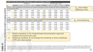
We retrieve the first five principal components from a large set of predictive variables and use them as the state variables. We report the cash flow betas of 25 size and book-to-market
portfolios. The first three panels vary only because we replace the 10-year PE ratio by either the 1-year PE ratio or the dividend yield. In Panel D, we replace the value spread by the
book-to-market spread and the market-to-book spread, following Liu and Zhang (2008). The standard errors of the differences in the cash flow betas between large and small, as well as
value and growth firms, are obtained through bootstrapping 10,000 realizations. We present results only for the 1963–2001 period.
Table 7: Cash flow betas with principal component analysis
βCF
Growth 2 3 4 Value Diff
Panel A: VAR variables include the excess equity market return, term spread, 10-year PE ratio,
value spread, credit spread, long-term corporate bond return, book-to-market ratio, 3-month T-bill
rate, inflation, corporate issuing activity, and stock variance.
Small 0.24 0.18 0.14 0.14 0.15 −0.09 [0.03]
2 0.16 0.13 0.12 0.09 0.11 −0.05 [0.03]
3 0.15 0.12 0.09 0.07 0.09 −0.06 [0.03]
4 0.14 0.09 0.09 0.04 0.06 −0.08 [0.03]
Large 0.07 0.07 0.05 0.06 0.04 −0.03 [0.03]
Diff −0.17 −0.11 −0.09 −0.08 −0.11
[0.04] [0.04] [0.03] [0.03] [0.03]
Panel B: VAR variables are the same as in Panel A except that the 10-year PE ratio is replaced by
the 1-year PE ratio.
Small 0.53 0.40 0.32 0.30 0.30 −0.23 [0.03]
2 0.43 0.31 0.26 0.21 0.23 −0.20 [0.03]
3 0.38 0.26 0.21 0.15 0.19 −0.19 [0.03]
4 0.35 0.23 0.19 0.12 0.14 −0.21 [0.03]
Large 0.22 0.17 0.13 0.11 0.09 −0.13 [0.03]
Diff −0.31 −0.23 −0.19 −0.19 −0.21
[0.04] [0.04] [0.03] [0.03] [0.03]
βCF
downward trend
from growth to value
βCF
larger downward
trend from growth to
value with substitutes
Michael-Paul James

34. Table
7:
Cash
flow
betas
with
principal
component
analysis
34
We retrieve the first five principal components from a large set of predictive variables and use them as the state variables. We report the cash flow betas of 25 size and book-to-market
portfolios. The first three panels vary only because we replace the 10-year PE ratio by either the 1-year PE ratio or the dividend yield. In Panel D, we replace the value spread by the
book-to-market spread and the market-to-book spread, following Liu and Zhang (2008). The standard errors of the differences in the cash flow betas between large and small, as well as
value and growth firms, are obtained through bootstrapping 10,000 realizations. We present results only for the 1963–2001 period.
Table 7: Cash flow betas with principal component analysis
Panel C: VAR variables are the same as in Panel A except that the 10-year PE ratio is replaced by
the dividend-yield.
Small 1.05 0.89 0.78 0.77 0.81 −0.24 [0.04]
2 0.93 0.80 0.74 0.67 0.74 −0.19 [0.04]
3 0.88 0.75 0.66 0.60 0.67 −0.21 [0.04]
4 0.79 0.69 0.62 0.53 0.61 −0.18 [0.04]
Large 0.60 0.58 0.49 0.47 0.49 −0.11 [0.04]
Diff −0.45 −0.31 −0.29 −0.30 −0.32
[0.06] [0.05] [0.05] [0.04] [0.04]
Panel D: VAR variables are the same as in Panel A except that the value spread is replaced by the
book-to market spread and the market-to-book spread.
Small 0.47 0.38 0.32 0.32 0.33 −0.14 [0.02]
2 0.41 0.30 0.26 0.25 0.28 −0.13 [0.02]
3 0.35 0.27 0.24 0.21 0.24 −0.11 [0.02]
4 0.31 0.26 0.22 0.19 0.21 −0.10 [0.02]
Large 0.20 0.20 0.17 0.15 0.16 −0.04 [0.02]
Diff −0.27 −0.18 −0.15 −0.17 −0.17
[0.03] [0.03] [0.03] [0.02] [0.02]
βCF
larger downward
trend from growth to
value with substitutes
Michael-Paul James

35. Table
8:
Cash
flow
betas
with
alternative
specifications
35
We study the cross-sectional pattern of cash flow betas when alternative specifications are used. In Panel A, we use the macro variables by Petkova (2004) that provide intuitive
interpretations on the Fama-French factors. In Panel B, we add variables shown by Lettau and Ludvigson (2001a, 2001b) and Ludvigson and Ng (2005) to exhibit good predictive power for
equity returns. Panel B uses quarterly data because these variables are available only at quarterly frequency. The standard errors of the differences in the cash flow betas between large
and small, as well as value and growth firms, are obtained through bootstrapping 10,000 realizations. We present results only for the 1963–2001 period.
Table 8: Cash flow betas with alternative specifications
βCF Growth 2 3 4 Value Diff
Panel A: VAR variables: excess equity market return, term yield, dividend yield, credit spread, and
risk-free rate.
Small 1.47 1.28 1.18 1.14 1.18 −0.29 [0.05]
2 1.39 1.23 1.13 1.08 1.12 −0.27 [0.05]
3 1.34 1.15 1.05 0.96 1.04 −0.30 [0.05]
4 1.21 1.07 0.99 0.93 1.02 −0.19 [0.05]
Large 0.93 0.91 0.77 0.74 0.77 −0.16 [0.04]
Diff −0.54 −0.37 −0.41 −0.40 −0.41
[0.07] [0.06] [0.05] [0.05] [0.05]
Panel B: VAR variables include excess equity market return, term spread, PE ratio, value spread,
cay, risk-premium factor, and volatility factor.
Small 0.48 0.43 0.40 0.40 0.44 −0.04 [0.07]
2 0.40 0.37 0.38 0.35 0.39 −0.01 [0.07]
3 0.35 0.34 0.32 0.33 0.36 0.01 [0.07]
4 0.33 0.32 0.32 0.32 0.35 0.02 [0.12]
Large 0.24 0.25 0.26 0.25 0.22 −0.02 [0.12]
Diff −0.24 −0.18 −0.14 −0.15 −0.22
[0.14] [0.14] [0.09] [0.09] [0.10]
Petkova motivated
macroeconomic
variables: excess
market return, term
spread, dividend yield,
credit spread
βCF
decrease from
growth to value
Lettau, Ludvigson, Ng
variables: cay,
risk-premium factor and
volatility factor
R2
increase to 14%
βCF
no trend
Michael-Paul James

36. Summary
36
● Cross sectional pattern of CF betas in Campbell and Vuolteenaho
seems to be a special case: value stocks do not have higher betas than
growth stocks for most specifications
○ Direct model of CF news
○ Bayesian model averaging approach
○ Principle component analysis
○ Special specifications motivated by economic reasoning
● Relative importance of CF and DR variances flips without clear pattern
● It is easy to draw opposite conclusions even with motivated variables
● Decompose directly modeled DR news, CF news, & residual news
● Mitigate model uncertainty with Bayesian model averaging approach
Michael-Paul James

37. Robustness
06
Further Robustness Checks
Industry portfolios
Post-1952 data
Other robustness checks
37
Michael-Paul James

38. Industry portfolios
38
● If cash flow beta is important to cost of equity, it is price in portfolios
● Tested against the Fama-French 48 industry portfolios
○ Lower CF betas tend to have higher returns
○ CF beta is significantly negative (wrong sign)
○ Higher CF betas should earn lower expected returns and have
lower costs of capital: opposite of CF beta risk interpretation.
Michael-Paul James

39. Post-1952 data and other checks
39
● Post 1952 data
○ Shift in variance after 1952, while CAPM breaks down in 1962
○ Clear decreasing cash flow beta trend from growth to value
■ Reversed from pre 1952 even with benchmark case
■ Trend is stable with other state variables
● Other checks that do not change core results
○ Magnitude of ρ ○ Data frequency
○ Additional VAR lags including 36 month rolling windows
○ Conditional betas
○ Use changes to state variables rather than levels
■ CF news acts like return itself, DR is small. Value lower βCF
Michael-Paul James

40. Conclusions
07
40
Michael-Paul James

41. Oops, Research Made a Boo Boo
41
● Directly modeling discount rate news and backing out cash flow news
adds residual news to the latter
○ The method has led to erroneous conclusions:
■ Larger relative DR variance
■ Value stocks earn higher returns due to higher βCF
■ βCF
is more important than total βtotal
○ DR news cannot be accurately estimated (low predictive power)
and backed out CF news inherits large misspecification error of DR
○ Modeled Treasury bonds reveals higher CF variance with no real CF
risk
○ Minor changes in predictive variables produce opposite results
Michael-Paul James

42. The Residual Effect
42
● Directly modeling cash flow news, discount rate news, and residual
○ Value firms have both lower modeled CF betas and DR betas, but
higher residual betas, indicating that the results in the current
literature are driven by the residual news.
Michael-Paul James

43. Motivating Discourse
43
● 373 citations on google scholar
● Undermines fundamental assumptions leading to new lines of inquiry
● Extensions
○ Ultimately what is residual news? Can it be measured? What are
its sources?
○ How does one motivate variables to accurately measure CF and DR
news betas?
○ How does investor sentiment interplay with cash flow
information?
Michael-Paul James

44. You are Amazing
Ask me all the questions you desire. I will do my best to answer honestly
and strive to grasp your intent and creativity.
44
Michael-Paul James