The term structure and interest rate
dynamics
Chapter 10
© 2016 CFA Institute. All rights reserved.
TABLE OF CONTENTS
01 INTRODUCTION
02 SPOT RATES AND FORWARD RATES
03 THE SWAP RATE CURVE
04 TRADITIONAL THEORIES OF THE TERM STRUCTURE OF
INTEREST RATES
05 MODERN TERM STRUCTURE MODELS
06 YIELD CURVE FACTOR MODELS
07 SUMMARY
1. INTRODUCTION
• Interest rates are both a barometer of the economy and an
instrument for its control.
• The term structure of interest rates—market interest rates
at various maturities—is a vital input into the valuation of
many financial products.
• The goal of this topic is to explain the term structure and
interest rate dynamics—that is, the process by which the
yields and prices of bonds evolve over time.
• The yield to maturity of the payment, denoted by r(T)Spot rate
2. SPOT RATES AND FORWARD RATES
At any point in time, the price of a risk-free single-unit payment (e.g.,
$1) at time T is called the “discount factor” r with maturity T, denoted
by P(T).
The spot curve represents the term structure of interest rates at
any point in time.
- The spot curve shows, for various maturities, the annualized return on an
option-free and default-risk-free zero-coupon bond with a single
payment of principal at maturity.
•
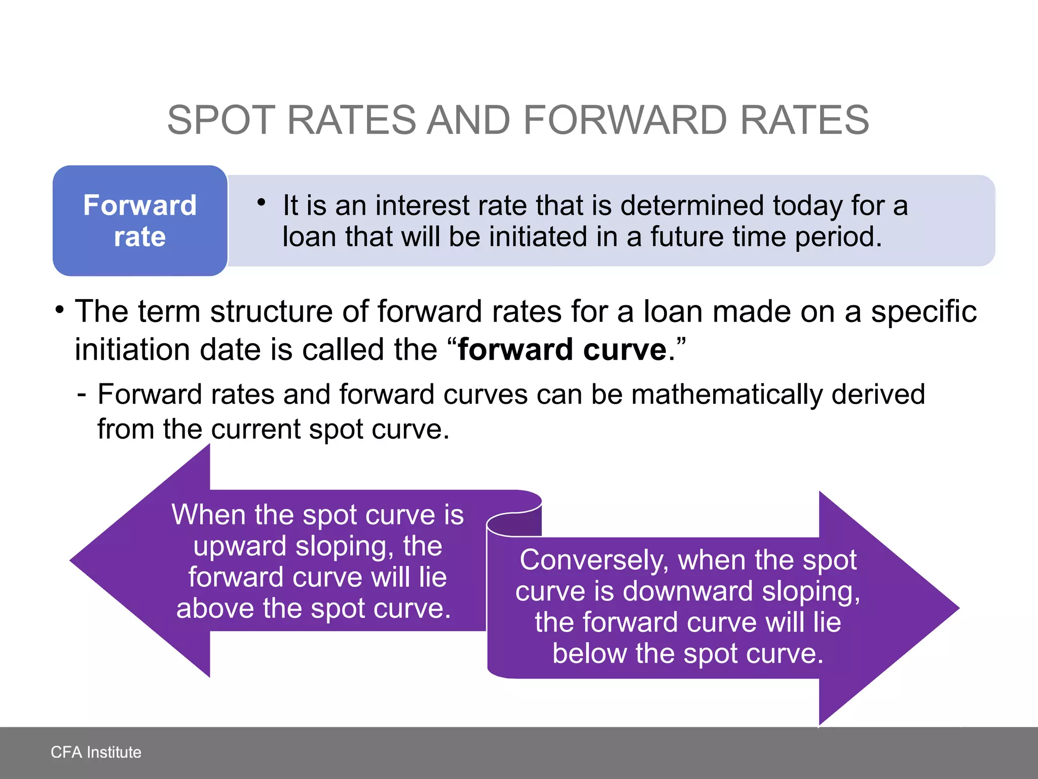
When the spot curve is
upward sloping, the
forward curve will lie
above the spot curve.
Conversely, when the spot
curve is downward sloping,
the forward curve will lie
below the spot curve.
• It is an interest rate that is determined today for a
loan that will be initiated in a future time period.
Forward
rate
SPOT RATES AND FORWARD RATES
• The term structure of forward rates for a loan made on a specific
initiation date is called the “forward curve.”
- Forward rates and forward curves can be mathematically derived
from the current spot curve.
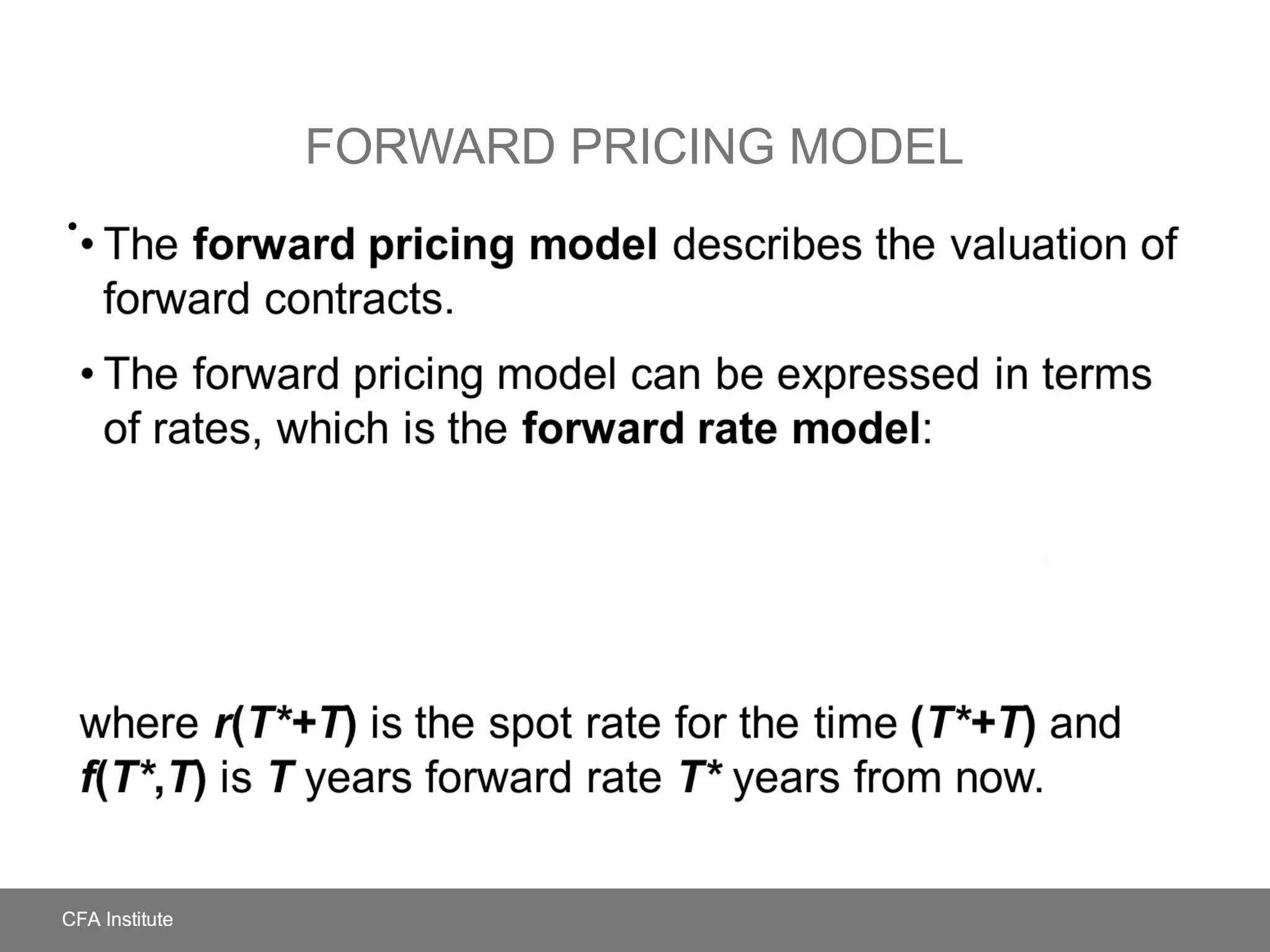
FORWARD PRICING MODEL
• The forward pricing model describes the valuation of
forward contracts.
• The forward pricing model can be expressed in terms
of rates, which is the forward rate model:
where r(T*+T) is the spot rate for the time (T*+T) and
f(T*,T) is T years forward rate T* years from now.
•
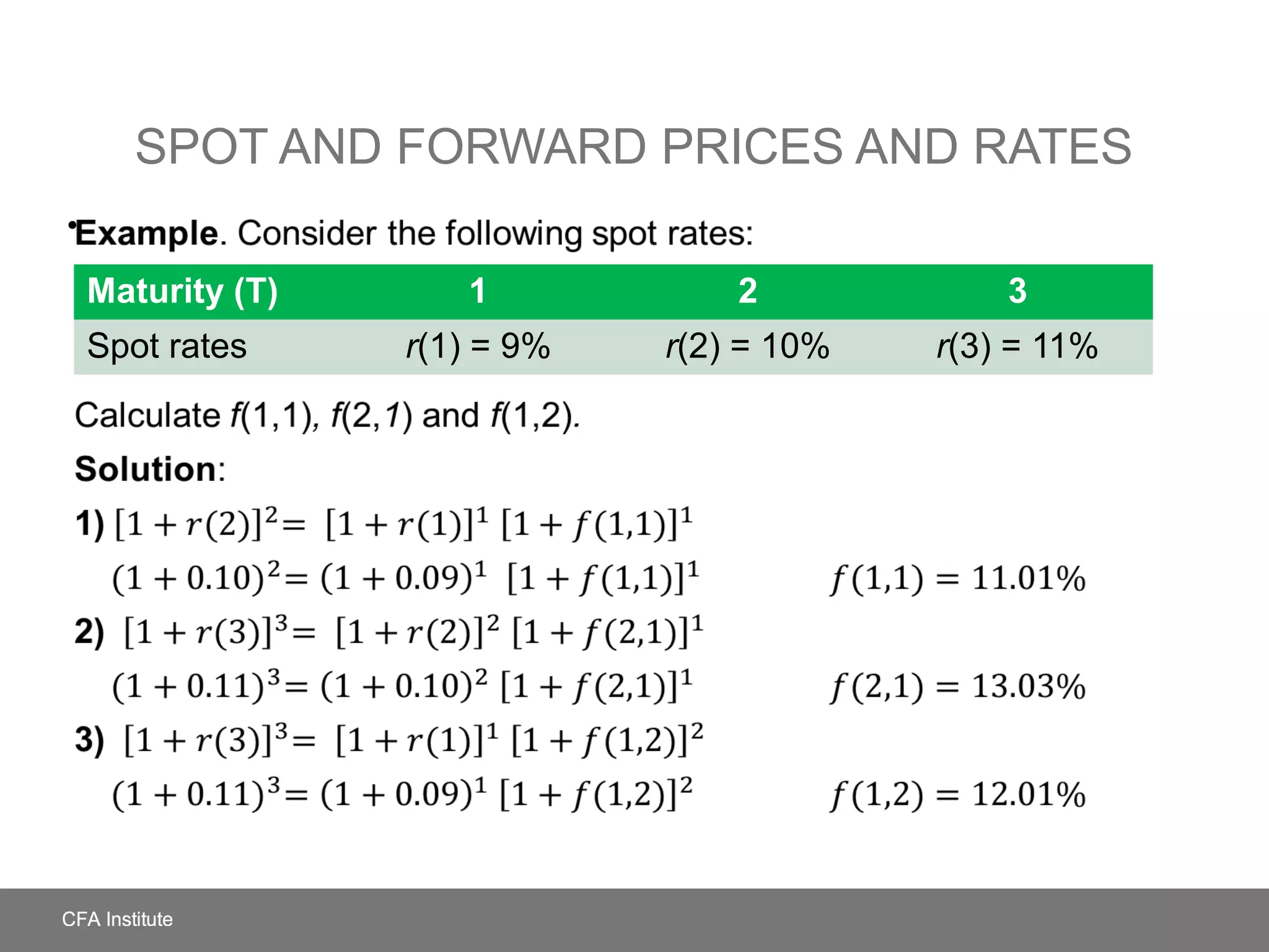
SPOT AND FORWARD PRICES AND RATES
Example. Consider the following spot rates:
Calculate f(1,1), f(2,1) and f(1,2).
Solution:
1)
2)
3)
•
Maturity (T) 1 2 3
Spot rates r(1) = 9% r(2) = 10% r(3) = 11%
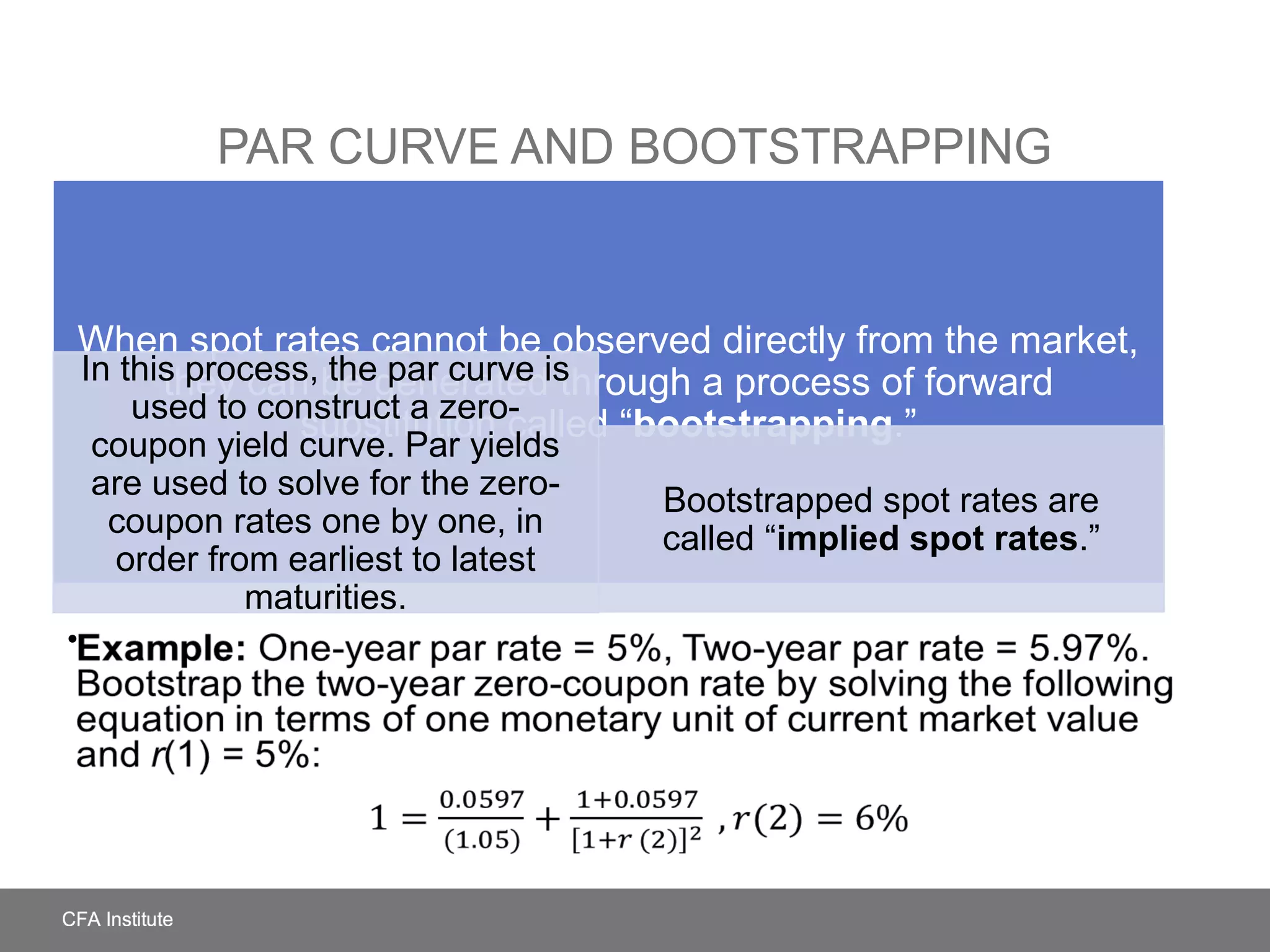
When spot rates cannot be observed directly from the market,
they can be generated through a process of forward
substitution called “bootstrapping.”
In this process, the par curve is
used to construct a zero-
coupon yield curve. Par yields
are used to solve for the zero-
coupon rates one by one, in
order from earliest to latest
maturities.
Bootstrapped spot rates are
called “implied spot rates.”
PAR CURVE AND BOOTSTRAPPING
Example: One-year par rate = 5%, Two-year par rate = 5.97%.
Bootstrap the two-year zero-coupon rate by solving the
following equation in terms of one monetary unit of current
market value and r(1) = 5%:
•
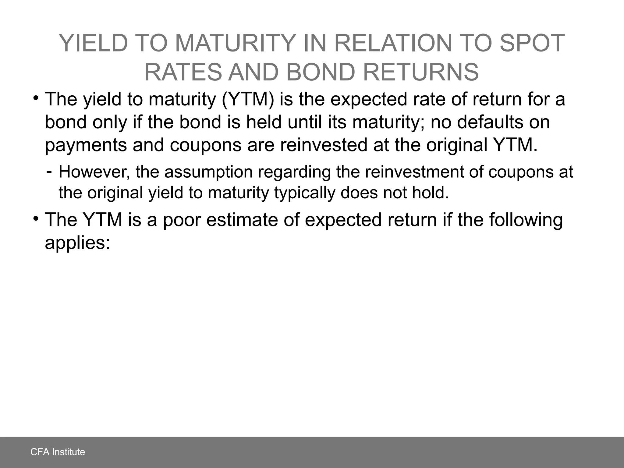
YIELD TO MATURITY IN RELATION TO SPOT
RATES AND BOND RETURNS
• The yield to maturity (YTM) is the expected rate of return for a
bond only if the bond is held until its maturity; no defaults on
payments and coupons are reinvested at the original YTM.
- However, the assumption regarding the reinvestment of coupons at
the original yield to maturity typically does not hold.
• The YTM is a poor estimate of expected return if the following
applies:
YIELD CURVE MOVEMENT AND
THE FORWARD CURVE
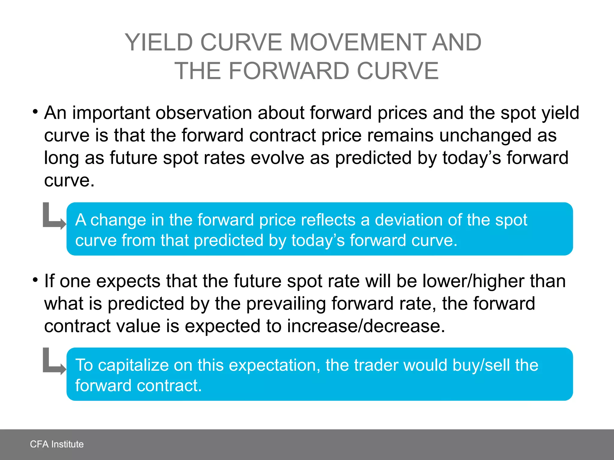
• An important observation about forward prices and the spot yield
curve is that the forward contract price remains unchanged as
long as future spot rates evolve as predicted by today’s forward
curve.
• If one expects that the future spot rate will be lower/higher than
what is predicted by the prevailing forward rate, the forward
contract value is expected to increase/decrease.
A change in the forward price reflects a deviation of the spot
curve from that predicted by today’s forward curve.
To capitalize on this expectation, the trader would buy/sell the
forward contract.
YIELD CURVE MOVEMENT AND
THE FORWARD CURVE
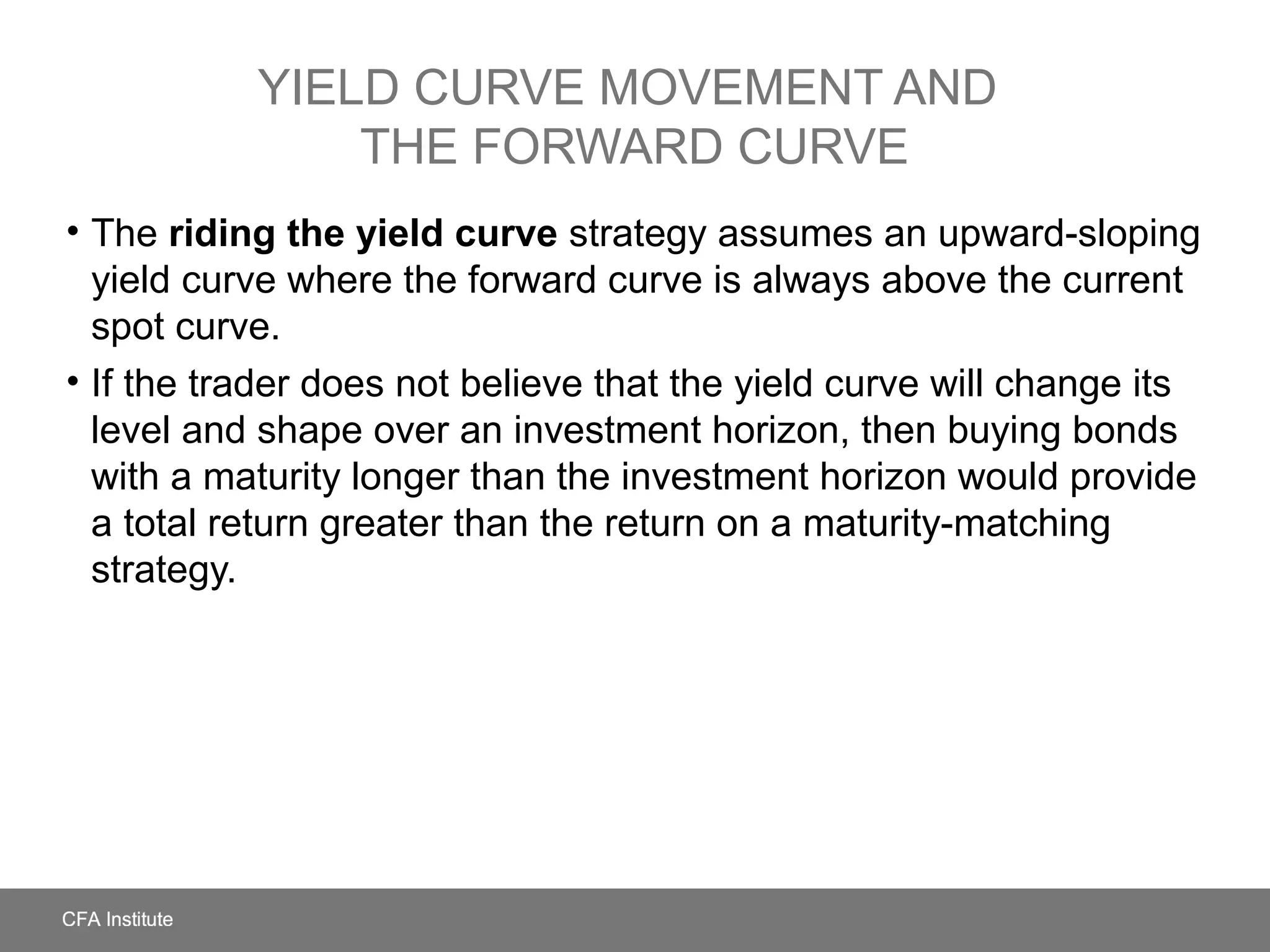
• The riding the yield curve strategy assumes an upward-sloping
yield curve where the forward curve is always above the current
spot curve.
• If the trader does not believe that the yield curve will change its
level and shape over an investment horizon, then buying bonds
with a maturity longer than the investment horizon would provide
a total return greater than the return on a maturity-matching
strategy.
3. The swap rate curve
Interest rate swaps are derivative contracts, where one
party exchanges fixed-rate interest payments for floating-
rate interest payments with another party.
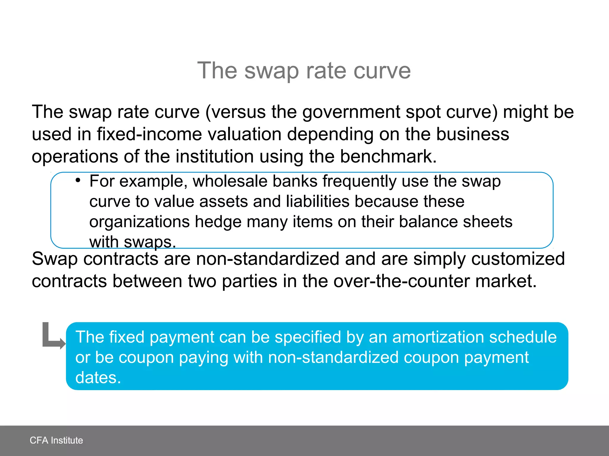
The swap rate curve
The swap rate curve (versus the government spot curve) might be
used in fixed-income valuation depending on the business
operations of the institution using the benchmark.
Swap contracts are non-standardized and are simply customized
contracts between two parties in the over-the-counter market.
●
For example, wholesale banks frequently use the swap
curve to value assets and liabilities because these
organizations hedge many items on their balance sheets
with swaps.
The fixed payment can be specified by an amortization schedule
or be coupon paying with non-standardized coupon payment
dates.
The swap SPREAD
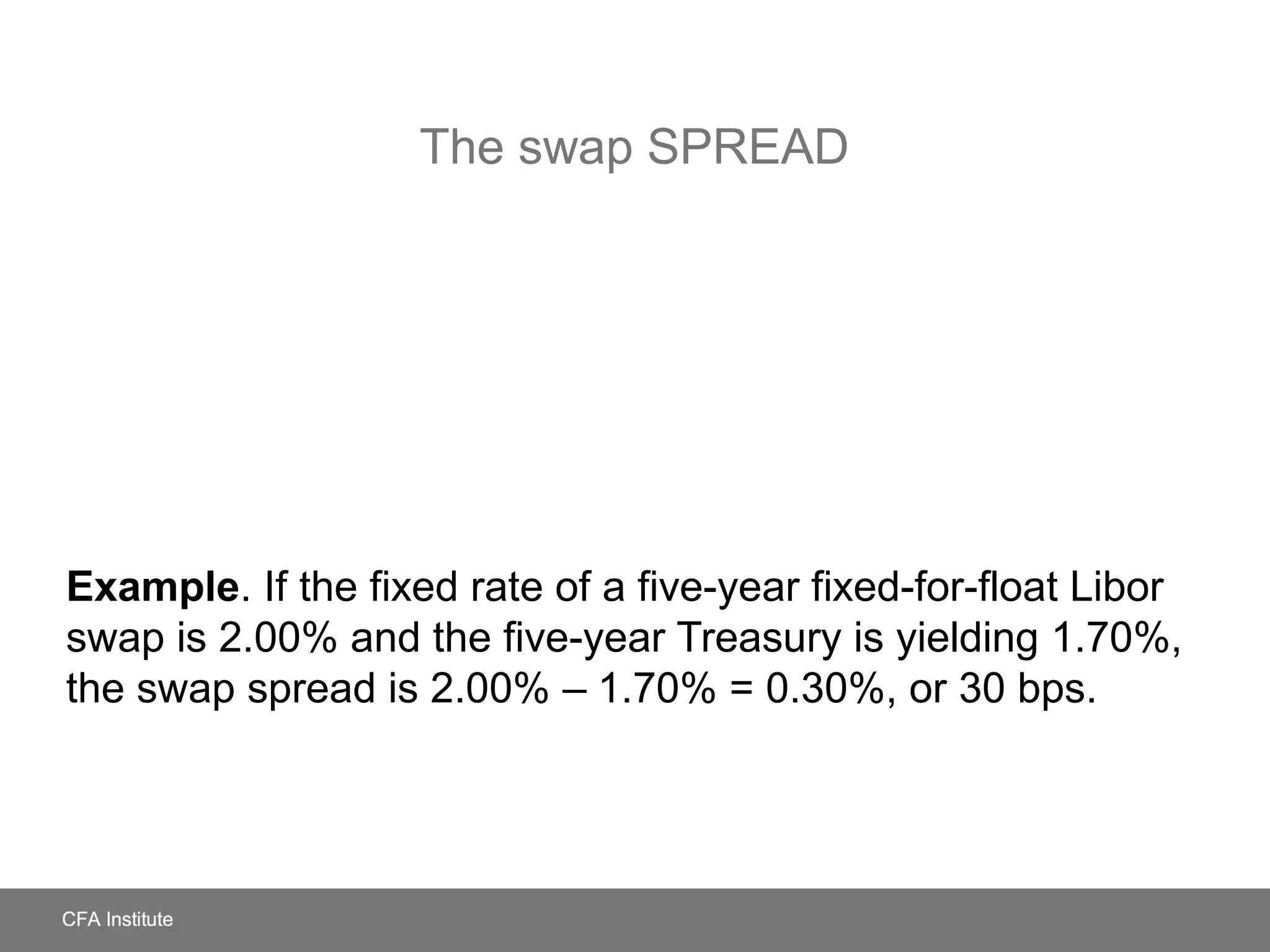
Example. If the fixed rate of a five-year fixed-for-float Libor
swap is 2.00% and the five-year Treasury is yielding 1.70%,
the swap spread is 2.00% 1.70% = 0.30%, or 30 bps.‒
The LIBOR/SWAP CURVE
A Libor/swap curve is probably the most widely used interest
rate curve because it is often viewed as reflecting the default
risk of private entities at a rating of about A1/A+, roughly the
equivalent of most commercial banks.
Z-SPREAD
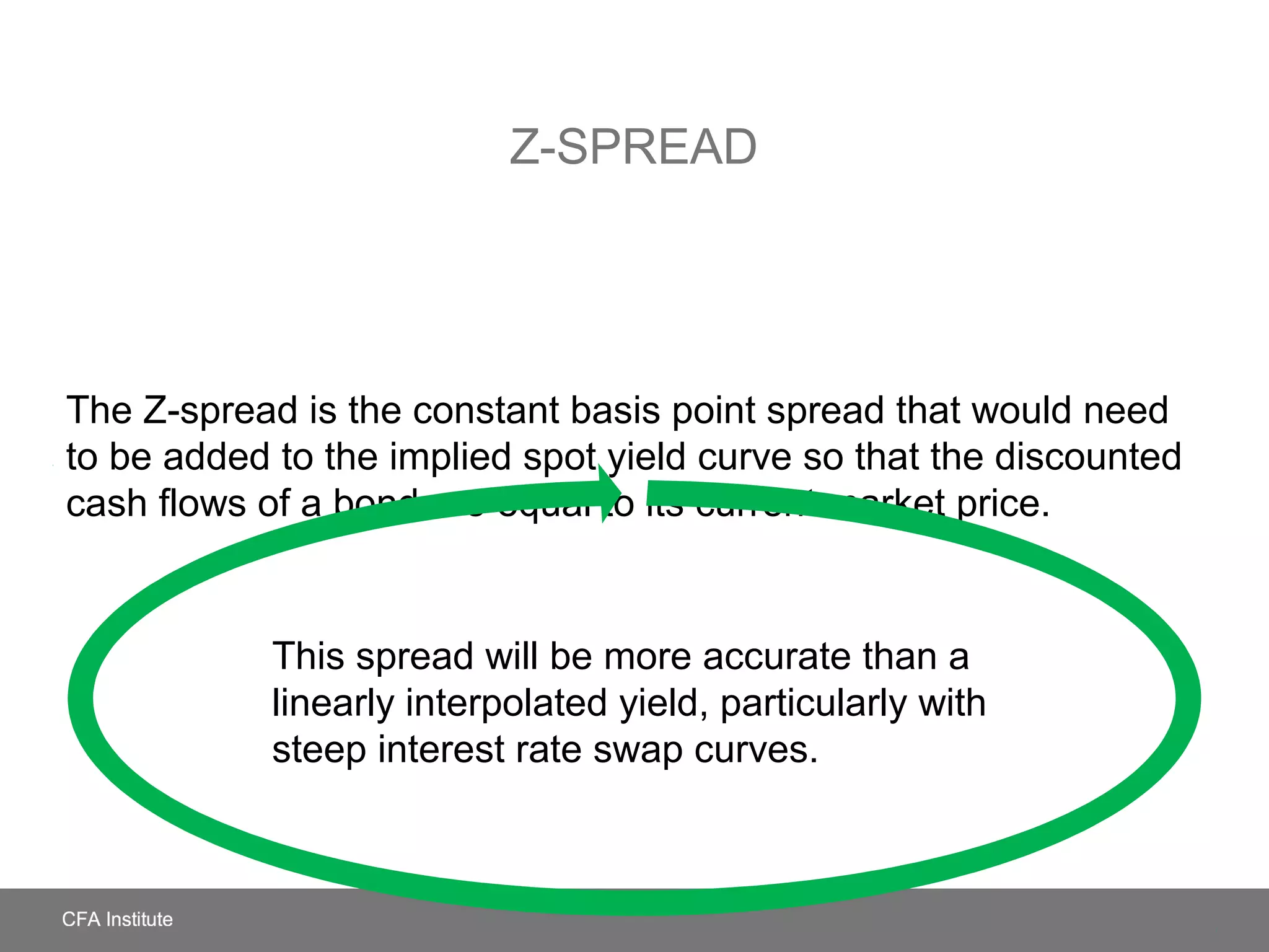
The Z-spread is the constant basis point spread that would need
to be added to the implied spot yield curve so that the discounted
cash flows of a bond are equal to its current market price.
This spread will be more accurate than a
linearly interpolated yield, particularly with
steep interest rate swap curves.
TED SPREAD AND LIBOR–OIS SPREAD
4. Traditional theories of the term structure of
interest rates
The pure expectations theory says that the forward rate is an
unbiased predictor of the future spot rate.
• Its broadest interpretation suggests that investors expect the
return for any investment horizon to be the same.
• The narrower interpretation—referred to as the local
expectations theory—suggests that the return will be the same
over a short-term horizon starting today.
PURE EXPECTATIONS THEORY
Under pure expectations theory, the shape of the yield curve
reflects the expectation about future short-term rates.
[ ] T
TTT ffzz
/1
,12,11 )1()1)(1()1( −+⋅⋅⋅++=+
The liquidity preference theory makes the following assertion:
• Liquidity premiums exist to compensate investors for the added
interest rate risk they face when lending long term, and these
premiums increase with maturity.
LIQUIDITY PREFERENCE THEORY
Thus, given an expectation of unchanging short-term spot rates,
liquidity preference theory predicts an upward-sloping yield
curve.
[ ] T
TTTT LfLfzz
/1
,122,11 )1()1)(1()1( ++⋅⋅⋅+++=+ −
SEGMENTED MARKETS AND
PREFERRED HABITAT THEORIES
5. Modern term structure models
• Modern term structure models provide quantitatively
precise descriptions of how interest rates evolve.
• Interest rate models attempt to capture the statistical
properties of interest rate movements.
Modern term structure models
• Equilibrium term structure models are models that seek to
describe the dynamics of the term structure using
fundamental economic variables that are assumed to affect
interest rates.
• They share the following characteristics:
CIR MODEL
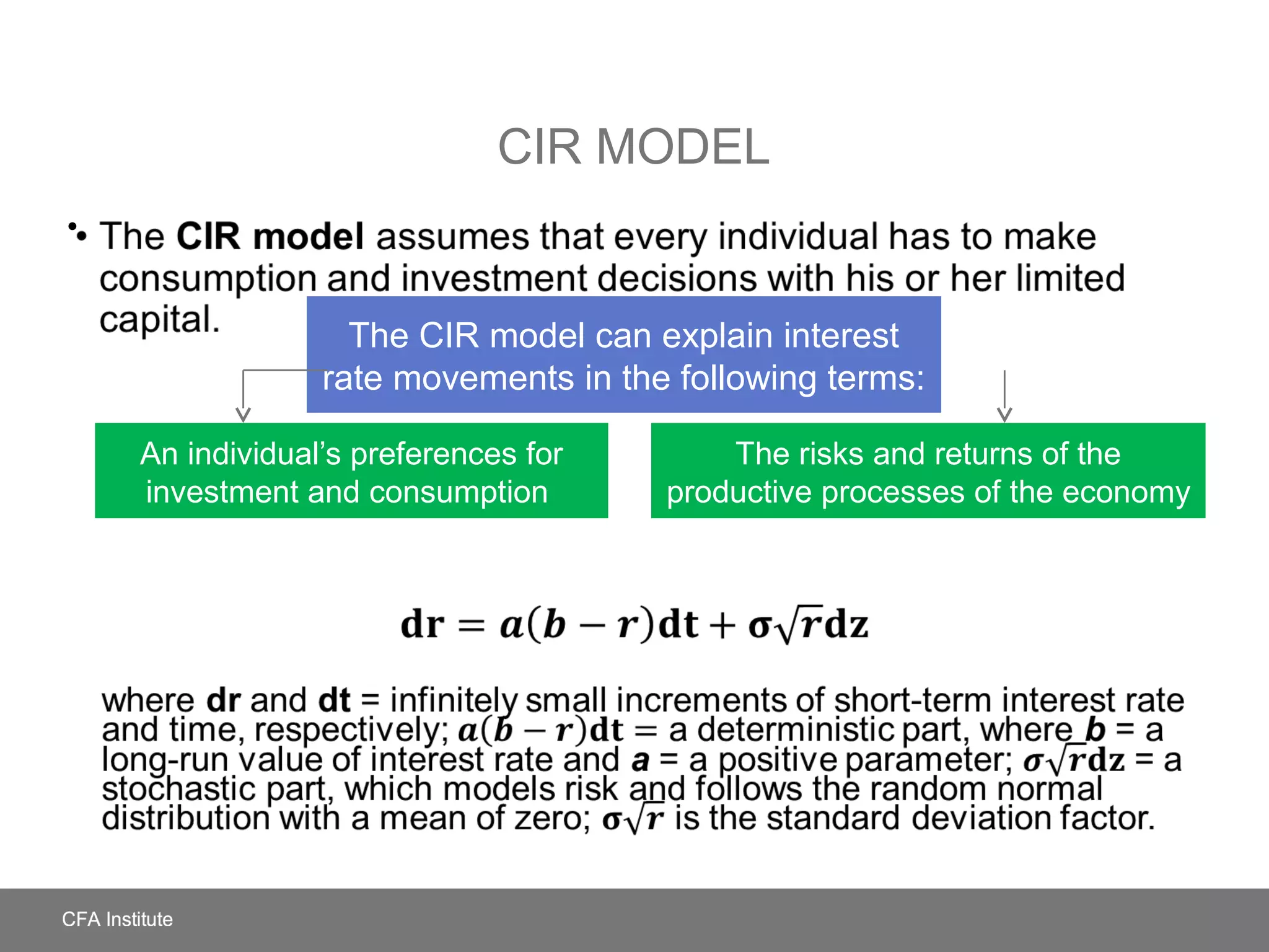
• The CIR model assumes that every individual has to make
consumption and investment decisions with his or her limited capital.
where dr and dt = infinitely small increments of short-term interest rate and
time, respectively; a deterministic part, where b = a long-run value of interest
rate and a = a positive parameter; = a stochastic part, which models risk and
follows the random normal distribution with a mean of zero; is the standard
deviation factor.
•
An individual’s preferences for
investment and consumption
The risks and returns of the
productive processes of the economy
The CIR model can explain interest
rate movements in the following terms:
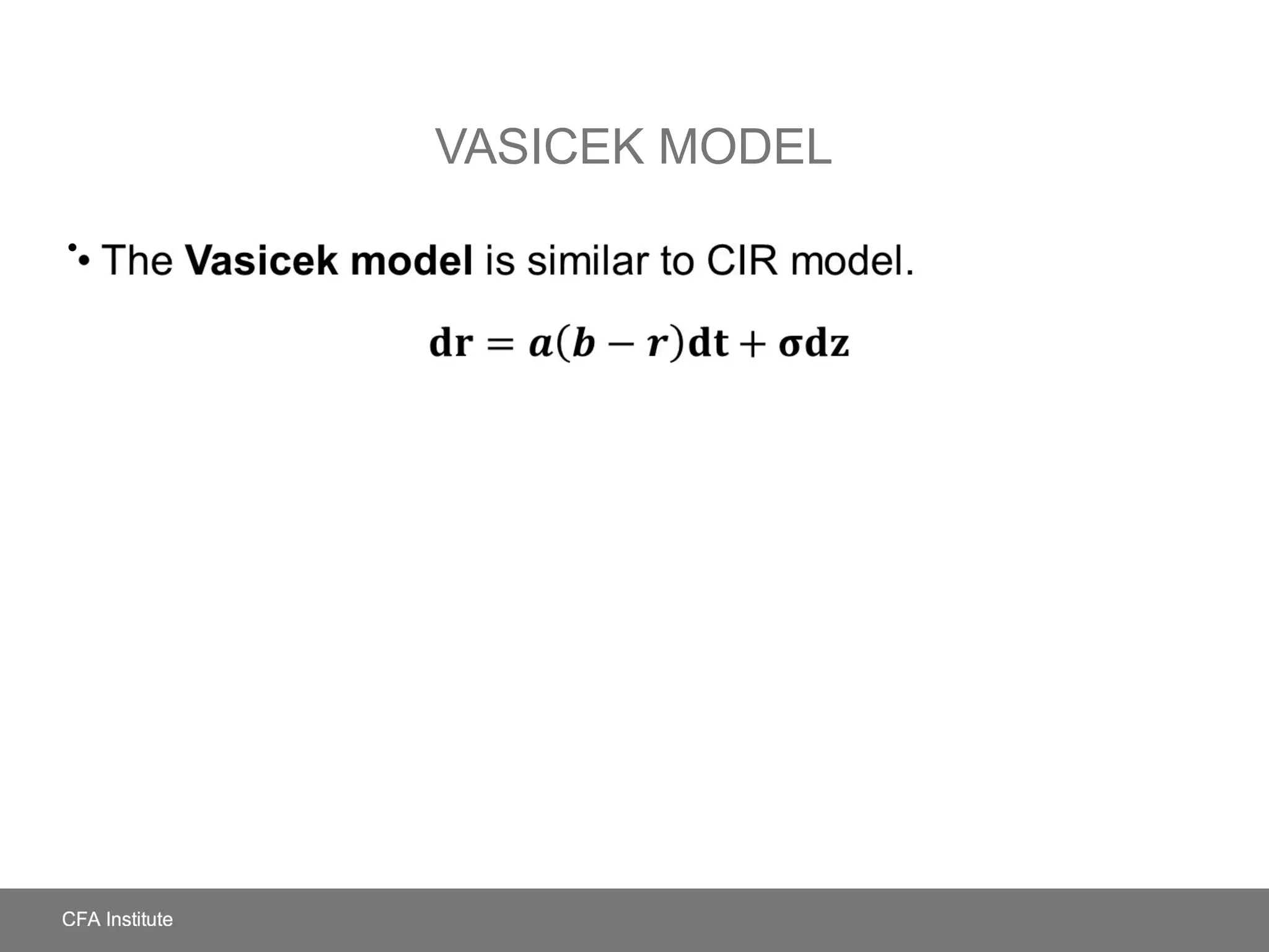
VASICEK MODEL
• The Vasicek model is similar to CIR model.•
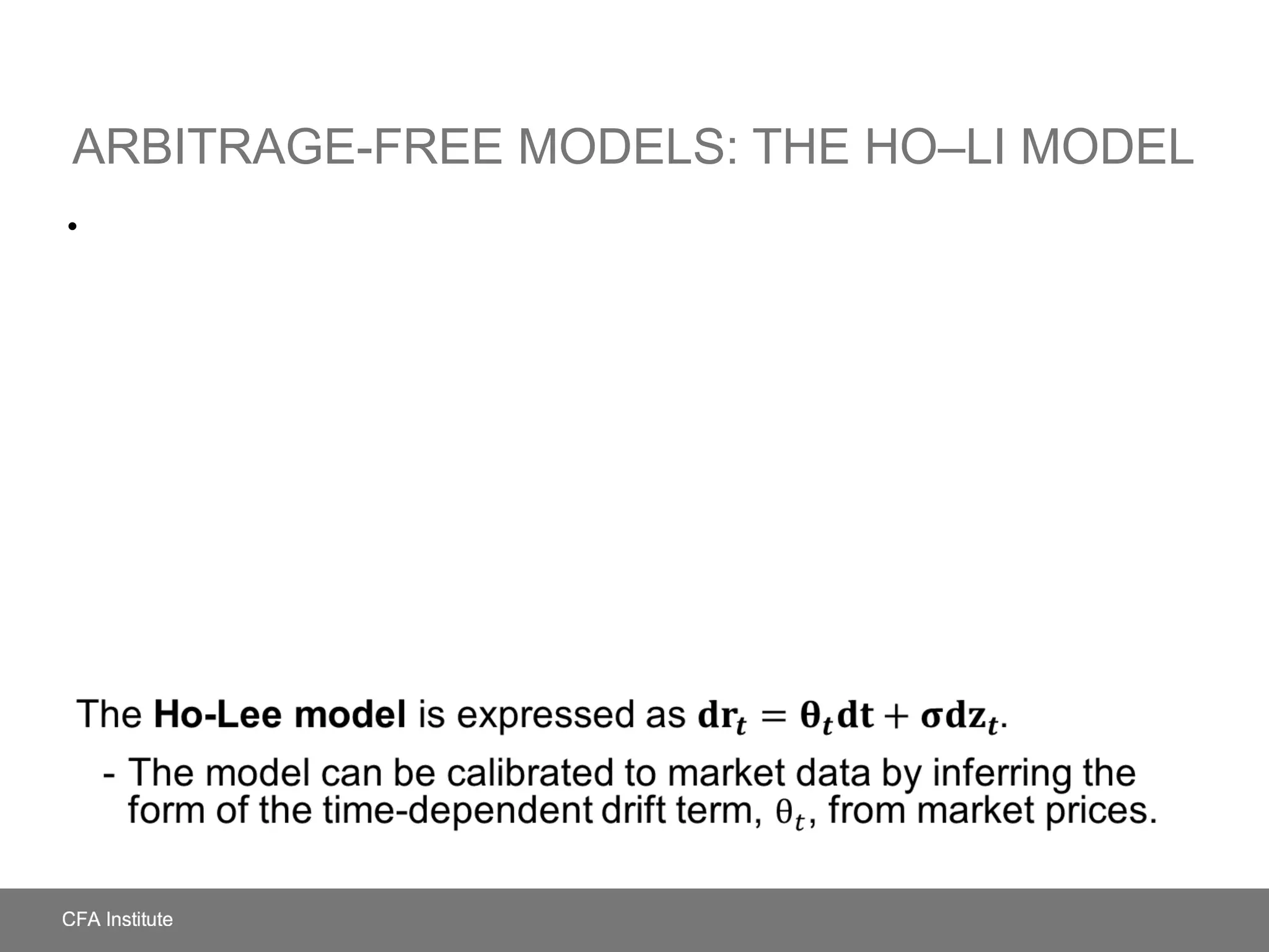
ARBITRAGE-FREE MODELS: THE HO–LI MODEL
The Ho-Lee model is expressed as .
- The model can be calibrated to market data by inferring the
form of the time-dependent drift term, , from market prices.
•
6. Yield curve factor models
• For active bond management, a bond investor may want to base
trades on a forecasted yield curve shape or may want to hedge
the yield curve risk on a bond portfolio.
• Litterman and Scheinkman (1991) decomposed yield curve
movements into a combination of three independent movements,
which they interpreted as level, steepness, and curvature.
FACTORS AFFECTING THE SHAPE
OF THE YIELD CURVE
• The approach that focuses on identifying the factors that best
explain historical variances is known as principal components
analysis (PCA).
Yield curve risk
Yield curve risk can be managed on the basis of several measures
of sensitivity to yield curve movements:
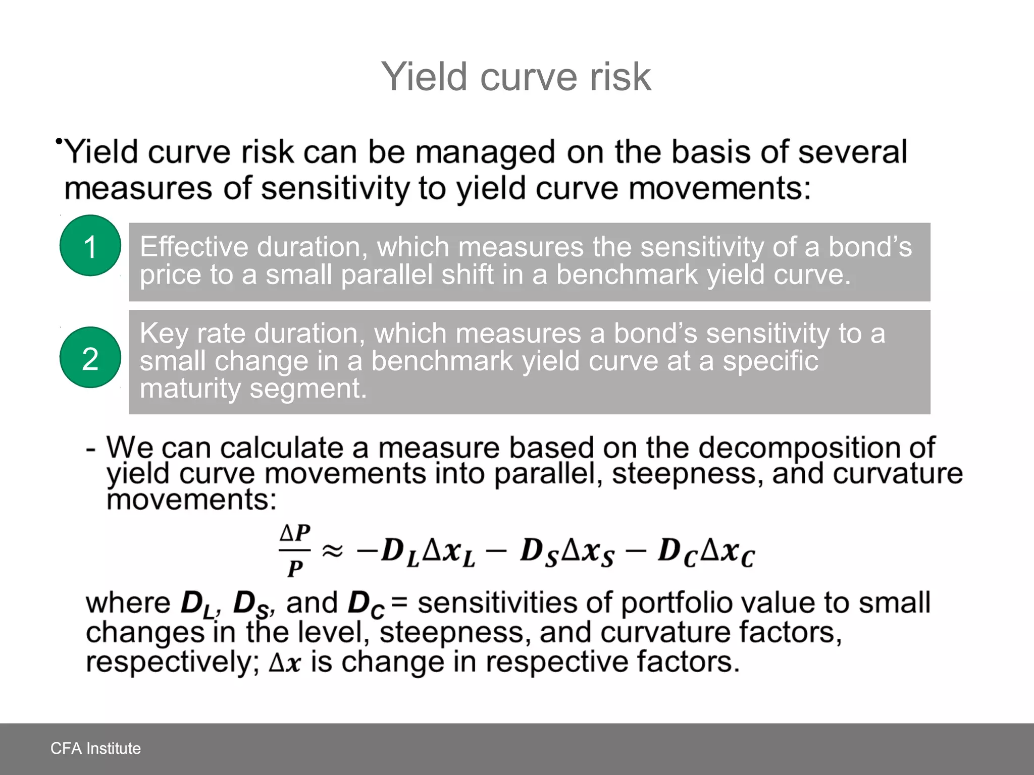
- We can calculate a measure based on the decomposition of yield curve
movements into parallel, steepness, and curvature movements:
where DL, DS, and DC = sensitivities of portfolio value to small changes
in the level, steepness, and curvature factors, respectively; is change in
respective factors.
•
Effective duration, which measures the sensitivity of a bond’s
price to a small parallel shift in a benchmark yield curve.
Key rate duration, which measures a bond’s sensitivity to a
small change in a benchmark yield curve at a specific
maturity segment.
1
2
THE MATURITY STRUCTURE OF
YIELD CURVE VOLATILITIES
• Quantifying interest rate volatilities is important for at least
two reasons:
• The term structure of interest rate volatilities is a
representation of the yield volatility of a zero-coupon bond for
every maturity of security.
• This volatility curve (or “vol”) or volatility term structure
measures yield curve risk.
- The volatility term structure typically shows that short-term rates
are more volatile than long-term rates.
7. SUMMARY
7. SUMMARY
SUMMARY
SUMMARY
SUMMARY

35 page the term structure and interest rate dynamics

  • 1.
    The term structureand interest rate dynamics Chapter 10 © 2016 CFA Institute. All rights reserved.
  • 2.
    TABLE OF CONTENTS 01INTRODUCTION 02 SPOT RATES AND FORWARD RATES 03 THE SWAP RATE CURVE 04 TRADITIONAL THEORIES OF THE TERM STRUCTURE OF INTEREST RATES 05 MODERN TERM STRUCTURE MODELS 06 YIELD CURVE FACTOR MODELS 07 SUMMARY
  • 3.
    1. INTRODUCTION • Interestrates are both a barometer of the economy and an instrument for its control. • The term structure of interest rates—market interest rates at various maturities—is a vital input into the valuation of many financial products. • The goal of this topic is to explain the term structure and interest rate dynamics—that is, the process by which the yields and prices of bonds evolve over time.
  • 4.
    • The yieldto maturity of the payment, denoted by r(T)Spot rate 2. SPOT RATES AND FORWARD RATES At any point in time, the price of a risk-free single-unit payment (e.g., $1) at time T is called the “discount factor” r with maturity T, denoted by P(T). The spot curve represents the term structure of interest rates at any point in time. - The spot curve shows, for various maturities, the annualized return on an option-free and default-risk-free zero-coupon bond with a single payment of principal at maturity. •
  • 5.
    When the spotcurve is upward sloping, the forward curve will lie above the spot curve. Conversely, when the spot curve is downward sloping, the forward curve will lie below the spot curve. • It is an interest rate that is determined today for a loan that will be initiated in a future time period. Forward rate SPOT RATES AND FORWARD RATES • The term structure of forward rates for a loan made on a specific initiation date is called the “forward curve.” - Forward rates and forward curves can be mathematically derived from the current spot curve.
  • 6.
    FORWARD PRICING MODEL •The forward pricing model describes the valuation of forward contracts. • The forward pricing model can be expressed in terms of rates, which is the forward rate model: where r(T*+T) is the spot rate for the time (T*+T) and f(T*,T) is T years forward rate T* years from now. •
  • 7.
    SPOT AND FORWARDPRICES AND RATES Example. Consider the following spot rates: Calculate f(1,1), f(2,1) and f(1,2). Solution: 1) 2) 3) • Maturity (T) 1 2 3 Spot rates r(1) = 9% r(2) = 10% r(3) = 11%
  • 8.
    When spot ratescannot be observed directly from the market, they can be generated through a process of forward substitution called “bootstrapping.” In this process, the par curve is used to construct a zero- coupon yield curve. Par yields are used to solve for the zero- coupon rates one by one, in order from earliest to latest maturities. Bootstrapped spot rates are called “implied spot rates.” PAR CURVE AND BOOTSTRAPPING Example: One-year par rate = 5%, Two-year par rate = 5.97%. Bootstrap the two-year zero-coupon rate by solving the following equation in terms of one monetary unit of current market value and r(1) = 5%: •
  • 9.
    YIELD TO MATURITYIN RELATION TO SPOT RATES AND BOND RETURNS • The yield to maturity (YTM) is the expected rate of return for a bond only if the bond is held until its maturity; no defaults on payments and coupons are reinvested at the original YTM. - However, the assumption regarding the reinvestment of coupons at the original yield to maturity typically does not hold. • The YTM is a poor estimate of expected return if the following applies:
  • 10.
    YIELD CURVE MOVEMENTAND THE FORWARD CURVE • An important observation about forward prices and the spot yield curve is that the forward contract price remains unchanged as long as future spot rates evolve as predicted by today’s forward curve. • If one expects that the future spot rate will be lower/higher than what is predicted by the prevailing forward rate, the forward contract value is expected to increase/decrease. A change in the forward price reflects a deviation of the spot curve from that predicted by today’s forward curve. To capitalize on this expectation, the trader would buy/sell the forward contract.
  • 11.
    YIELD CURVE MOVEMENTAND THE FORWARD CURVE • The riding the yield curve strategy assumes an upward-sloping yield curve where the forward curve is always above the current spot curve. • If the trader does not believe that the yield curve will change its level and shape over an investment horizon, then buying bonds with a maturity longer than the investment horizon would provide a total return greater than the return on a maturity-matching strategy.
  • 12.
    3. The swaprate curve Interest rate swaps are derivative contracts, where one party exchanges fixed-rate interest payments for floating- rate interest payments with another party.
  • 13.
    The swap ratecurve The swap rate curve (versus the government spot curve) might be used in fixed-income valuation depending on the business operations of the institution using the benchmark. Swap contracts are non-standardized and are simply customized contracts between two parties in the over-the-counter market. ● For example, wholesale banks frequently use the swap curve to value assets and liabilities because these organizations hedge many items on their balance sheets with swaps. The fixed payment can be specified by an amortization schedule or be coupon paying with non-standardized coupon payment dates.
  • 14.
    The swap SPREAD Example.If the fixed rate of a five-year fixed-for-float Libor swap is 2.00% and the five-year Treasury is yielding 1.70%, the swap spread is 2.00% 1.70% = 0.30%, or 30 bps.‒
  • 15.
    The LIBOR/SWAP CURVE ALibor/swap curve is probably the most widely used interest rate curve because it is often viewed as reflecting the default risk of private entities at a rating of about A1/A+, roughly the equivalent of most commercial banks.
  • 16.
    Z-SPREAD The Z-spread isthe constant basis point spread that would need to be added to the implied spot yield curve so that the discounted cash flows of a bond are equal to its current market price. This spread will be more accurate than a linearly interpolated yield, particularly with steep interest rate swap curves.
  • 17.
    TED SPREAD ANDLIBOR–OIS SPREAD
  • 18.
    4. Traditional theoriesof the term structure of interest rates
  • 19.
    The pure expectationstheory says that the forward rate is an unbiased predictor of the future spot rate. • Its broadest interpretation suggests that investors expect the return for any investment horizon to be the same. • The narrower interpretation—referred to as the local expectations theory—suggests that the return will be the same over a short-term horizon starting today. PURE EXPECTATIONS THEORY Under pure expectations theory, the shape of the yield curve reflects the expectation about future short-term rates. [ ] T TTT ffzz /1 ,12,11 )1()1)(1()1( −+⋅⋅⋅++=+
  • 20.
    The liquidity preferencetheory makes the following assertion: • Liquidity premiums exist to compensate investors for the added interest rate risk they face when lending long term, and these premiums increase with maturity. LIQUIDITY PREFERENCE THEORY Thus, given an expectation of unchanging short-term spot rates, liquidity preference theory predicts an upward-sloping yield curve. [ ] T TTTT LfLfzz /1 ,122,11 )1()1)(1()1( ++⋅⋅⋅+++=+ −
  • 21.
  • 22.
    5. Modern termstructure models • Modern term structure models provide quantitatively precise descriptions of how interest rates evolve. • Interest rate models attempt to capture the statistical properties of interest rate movements.
  • 23.
    Modern term structuremodels • Equilibrium term structure models are models that seek to describe the dynamics of the term structure using fundamental economic variables that are assumed to affect interest rates. • They share the following characteristics:
  • 24.
    CIR MODEL • TheCIR model assumes that every individual has to make consumption and investment decisions with his or her limited capital. where dr and dt = infinitely small increments of short-term interest rate and time, respectively; a deterministic part, where b = a long-run value of interest rate and a = a positive parameter; = a stochastic part, which models risk and follows the random normal distribution with a mean of zero; is the standard deviation factor. • An individual’s preferences for investment and consumption The risks and returns of the productive processes of the economy The CIR model can explain interest rate movements in the following terms:
  • 25.
    VASICEK MODEL • TheVasicek model is similar to CIR model.•
  • 26.
    ARBITRAGE-FREE MODELS: THEHO–LI MODEL The Ho-Lee model is expressed as . - The model can be calibrated to market data by inferring the form of the time-dependent drift term, , from market prices. •
  • 27.
    6. Yield curvefactor models • For active bond management, a bond investor may want to base trades on a forecasted yield curve shape or may want to hedge the yield curve risk on a bond portfolio. • Litterman and Scheinkman (1991) decomposed yield curve movements into a combination of three independent movements, which they interpreted as level, steepness, and curvature.
  • 28.
    FACTORS AFFECTING THESHAPE OF THE YIELD CURVE • The approach that focuses on identifying the factors that best explain historical variances is known as principal components analysis (PCA).
  • 29.
    Yield curve risk Yieldcurve risk can be managed on the basis of several measures of sensitivity to yield curve movements: - We can calculate a measure based on the decomposition of yield curve movements into parallel, steepness, and curvature movements: where DL, DS, and DC = sensitivities of portfolio value to small changes in the level, steepness, and curvature factors, respectively; is change in respective factors. • Effective duration, which measures the sensitivity of a bond’s price to a small parallel shift in a benchmark yield curve. Key rate duration, which measures a bond’s sensitivity to a small change in a benchmark yield curve at a specific maturity segment. 1 2
  • 30.
    THE MATURITY STRUCTUREOF YIELD CURVE VOLATILITIES • Quantifying interest rate volatilities is important for at least two reasons: • The term structure of interest rate volatilities is a representation of the yield volatility of a zero-coupon bond for every maturity of security. • This volatility curve (or “vol”) or volatility term structure measures yield curve risk. - The volatility term structure typically shows that short-term rates are more volatile than long-term rates.
  • 31.
  • 32.
  • 33.
  • 34.
  • 35.

Editor's Notes

  • #2 <number>
  • #4 1. Introduction <number>
  • #5 2. The term structure and interest rate dynamics LOS: Describe relationships among spot rates, forward rates, yield to maturity, expected and realized returns on bonds, and the shape of the yield curve. The discount factor, P(T), and the spot rate, r(T), for a range of maturities in years T > 0 are called the “discount function” and the “spot yield curve” (or, more simply, spot curve), respectively. Note that the discount function completely identifies the spot curve, and vice versa. The discount function and the spot curve contain the same set of information about the time value of money. <number>
  • #6 2. The term structure and interest rate dynamics LOS: Describe relationships among spot rates, forward rates, yield to maturity, expected and realized returns on bonds, and the shape of the yield curve. The relationship between spot and forward curves is a reflection of the basic mathematical truth that when the average is rising (falling), the marginal data point must be above (below) the average. In this case, the spot curve represents an average over a whole time period and the forward rates represent the marginal changes between future time periods. <number>
  • #7 2. The term structure and interest rate dynamics LOS: Describe the forward pricing and forward rate models and calculate forward and spot prices and rates using those models. The forward pricing model equation is P(M+T) = P(M) × F(M,T), where P(M + T) and P(M) are discount factors for period T + M and M respectively. The formula can be used to derive both spot and forward rates. <number>
  • #8 2. The term structure and interest rate dynamics LOS: Describe the forward pricing and forward rate models and calculate forward and spot prices and rates using those models. There could be two interpretations of the forward rate model equalities—for example, for scenario 1 in the slide: The reinvestment rate that would make an investor indifferent between buying an two-year zero-coupon bond or investing in a one-year zero-coupon bond and, at maturity, reinvesting the proceeds for one year. In this sense, the forward rate can be viewed as a type of breakeven interest rate. The two-year rate that can be locked in today by buying an one-year zero-coupon bond rather than investing in a one-year zero-coupon bond and, when it matures, reinvesting the proceeds in a zero-coupon instrument that matures in one year. In this sense, the forward rate can be viewed as a rate that can be locked in by extending maturity by one year. <number>
  • #9 2. The term structure and interest rate dynamics LOS: Describe the forward pricing and forward rate models and calculate forward and spot prices and rates using those models. The par curve represents the yields to maturity on coupon-paying government bonds, priced at par, over a range of maturities. In practice, recently issued (“on the run”) bonds are typically used to create the par curve because new issues are typically priced at or close to par. <number>
  • #10 2. The term structure and interest rate dynamics LOS: Describe the forward pricing and forward rate models and calculate forward and spot prices and rates using those models. If either (1) or (2) is the case, the reinvestment of coupons would not be expected to be at the assumed rate (YTM). Case (3) implies that actual cash flows may differ from those assumed in the YTM calculation, and in case (4), the exercise of an embedded option would, in general, result in a holding period that is shorter than the bond’s original maturity. <number>
  • #11 2. The term structure and interest rate dynamics LOS: Describe the assumptions concerning the evolution of spot rates in relation to forward rates implicit in active bond portfolio management. If the spot rate curve is unchanged, then each bond “rolls down” the curve and earns the forward rate. If any one of the investor’s expected future spot rates is lower than a quoted forward rate for the same maturity, then (all else being equal) the investor would perceive the bond to be undervalued in the sense that the market is effectively discounting the bond’s payments at a higher rate than the investor is and the bond’s market price is below the intrinsic value perceived by the investor. <number>
  • #12 2. The term structure and interest rate dynamics LOS: Describe the strategy of riding the yield curve. When the yield curve slopes upward, as a bond approaches maturity, or “rolls down the yield curve,” it is valued at successively lower yields and higher prices. Using this strategy, a bond can be held for a period of time as it appreciates in price and then sold before maturity to realize a higher return. <number>
  • #13 3. The swap rate curve LOS: Explain the swap rate curve, and why and how market participants use it in valuation. Examples of floating reference rates are three-month or six-month dollar Libor (London Interbank Offered Rate), euro-denominated Euribor (European Interbank Offered Rate), and yen-denominated Tibor (Tokyo Interbank Offered Rate). The swap curve is based on so-called par swaps, in which the fixed rates are set so that no money is exchanged at contract initiation—the present values of the fixed-rate and benchmark floating-rate legs being equal. The swap curve is a type of par curve. <number>
  • #14 3. The swap rate curve LOS: Explain the swap rate curve, and why and how market participants use it in valuation. To price a swap, we need to determine the present value of cash flows for each leg of the transaction. In an interest rate swap, the fixed leg is fairly straightforward because the cash flows are specified by the coupon rate set at the time of the agreement. Pricing the floating leg is more complex because, by definition, the cash flows change with future changes in interest rates. The forward rate for each floating payment date is calculated by using the forward curves. <number>
  • #15 3. The swap rate curve LOS: Calculate and interpret the swap spread for a default-free bond. For euro-denominated swaps, the government yield used as a benchmark is most frequently bunds (German government bonds) with the same maturity. Gilts (UK government bonds) are used as a benchmark in the United Kingdom. <number>
  • #16 3. The swap rate curve LOS: Calculate and interpret the swap spread for a default-free bond. The term “swap spread” is sometimes also used as a reference to a bond’s basis point spread over the interest rate swap curve and is a measure of the credit and/or liquidity risk of a bond. <number>
  • #17 3. The swap rate curve LOS: Describe the Z-spread. <number>
  • #18 3. The swap rate curve LOS: Describe the TED and Libor– OIS spreads. TED is an acronym formed from US T-bill and ED, the ticker symbol for the eurodollar futures contract. An increase (decrease) in the TED spread is a sign that lenders believe the risk of default on interbank loans is increasing (decreasing). An OIS is an interest rate swap in which the periodic floating rate of the swap is equal to the geometric average of an overnight rate (or overnight index rate) over every day of the payment period. The index rate is typically the rate for overnight unsecured lending between banks—for example, the federal funds rate for US dollars, Eonia (Euro OverNight Index Average) for euros, and Sonia (Sterling OverNight Index Average) for sterling. <number>
  • #19 4. Traditional theories of the term structure of interest rates LOS: Explain traditional theories of the term structure of interest rates and describe the implications of each theory for forward rates and the shape of the yield curve. The pure expectations theory is also known as the unbiased expectations theory. <number>
  • #20 4. Traditional theories of the term structure of interest rates LOS: Explain traditional theories of the term structure of interest rates and describe the implications of each theory for forward rates and the shape of the yield curve. The predictions of the unbiased expectations theory are consistent with the assumption of risk neutrality. Because forward rates are not perfect predictors of future interest rates, the pure expectations theory neglects the risks (interest rate risk and reinvestment risk) associated with investing in Treasury securities. Advocates of the pure expectations theory argue that forward rates are the market’s consensus of future interest rates. <number>
  • #21 4. Traditional theories of the term structure of interest rates LOS: Explain traditional theories of the term structure of interest rates and describe the implications of each theory for forward rates and the shape of the yield curve. Although downward-sloping or hump-shaped yield curves may sometimes occur, the existence of liquidity premiums implies that the yield curve will typically be upward sloping. <number>
  • #22 4. Traditional theories of the term structure of interest rates LOS: Explain traditional theories of the term structure of interest rates and describe the implications of each theory for forward rates and the shape of the yield curve. The preferred habitat theory is based on the realistic notion that agents and institutions will accept additional risk in return for additional expected returns. In accepting elements of both the segmented markets theory and the unbiased expectations theory yet rejecting their extreme polar positions, the preferred habitat theory moves closer to explaining real-world phenomena. <number>
  • #23 5. Modern term structure models LOS: Describe modern term structure models and how they are used. <number>
  • #24 5. Modern term structure models LOS: Describe modern term structure models and how they are used. One-factor models assume that a single observable factor (sometimes called a “state variable”) drives all yield curve movements. Both the Vasicek and CIR models assume a single factor, the short-term interest rate, r. This approach is plausible because empirically, parallel shifts are often found to explain more than 90% of yield changes. In contrast, multifactor models may be able to model the curvature of a yield curve more accurately but at the cost of greater complexity. <number>
  • #25 5. Modern term structure models LOS: Describe modern term structure models and how they are used. The model shows how the short-term interest rate is related to the risks facing the productive processes of the economy. Assuming that an individual requires a term premium on the long-term rate, the model shows that the short-term rate can determine the entire term structure of interest rates and the valuation of interest rate–contingent claims. For simplicity of presentation, the formula in the slide assumes that the term premium of the CIR model is equal to zero. <number>
  • #26 5. Modern term structure models. LOS: Describe modern term structure models and how they are used. Because both the Vasicek model and the CIR model require the short-term rate to follow a certain process, the estimated yield curve may not match the observed yield curve. But if the parameters of the models are believed to be correct, then investors can use these models to determine mispricings. <number>
  • #27 5. Modern term structure models LOS: Describe modern term structure models and how they are used. Arbitrage-free models do not attempt to explain the observed yield curve. Instead, these models take the yield curve as given. For this reason, they are sometimes labeled as partial equilibrium models. The basic arbitrage-free concept can be used to solve much broader problems. These models can be extended to value many bond types, allowing for a term structure of volatilities, uncertain changes in the shape of the yield curve, adjustments for the credit risk of a bond, and much more. <number>
  • #28 6. Yield curve factor models LOS: Explain how a bond’s exposure to each of the factors driving the yield curve can be measured and how these exposures can be used to manage yield curve risks. The level movement refers to an upward or downward shift in the yield curve. The steepness movement refers to a non-parallel shift in the yield curve when either short-term rates change more than long-term rates or long-term rates change more than short-term rates. The curvature movement is a reference to movement in three segments of the yield curve: The short-term and long-term segments rise while the middle-term segment falls, or vice versa. <number>
  • #29 6. Yield curve factor models LOS: Explain how a bond’s exposure to each of the factors driving the yield curve can be measured and how these exposures can be used to manage yield curve risks. PCA creates a number of synthetic factors defined as (and calculated to be) statistically independent of each other; how these factors may be interpreted economically is a challenge to the researcher that can be addressed by relating movements in the factors (as we will call the principal components in this discussion) to movements in observable and easily understood variables. <number>
  • #30 6. Yield curve factor models LOS: Explain how a bond’s exposure to each of the factors driving the yield curve can be measured and how these exposures can be used to manage yield curve risks. Effective duration is used to measure the change in the level factor, whereas key rate duration is used to measure the change in steepness and curvature factors. <number>
  • #31 6. Yield curve factor models LOS: Explain the maturity structure of yield volatilities and their effect on price volatility. Interest rate volatility is not the same for all interest rates along the yield curve. Research indicates that short-term volatility is most strongly linked to uncertainty regarding monetary policy whereas long-term volatility is most strongly linked to uncertainty regarding the real economy and inflation. <number>
  • #32 LOS: Describe relationships among spot rates, forward rates, yield to maturity, expected and realized returns on bonds, and the shape of the yield curve. <number>
  • #33 LOS: Describe the forward pricing and forward rate models and calculate forward and spot prices and rates using those models. <number>
  • #34 LOS: Describe the assumptions concerning the evolution of spot rates in relation to forward rates implicit in active bond portfolio management. LOS: Explain the swap rate curve, and why and how market participants use it in valuation. LOS: Calculate and interpret the swap spread for a default-free bond. LOS: Describe the Z-spread. LOS: Describe the TED and Libor–OIS spreads. <number>
  • #35 LOS: Explain the maturity structure of yield volatilities and their effect on price volatility. <number>
  • #36 LOS: Explain traditional theories of the term structure of interest rates and describe the implications of each theory for forward rates and the shape of the yield curve. LOS: Describe modern term structure models and how they are used. LOS: Explain how a bond’s exposure to each of the factors driving the yield curve can be measured and how these exposures can be used to manage yield curve risks. LOS: Explain the maturity structure of yield volatilities and their effect on price volatility. <number>