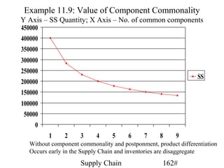
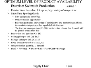
Downloaded 45 times

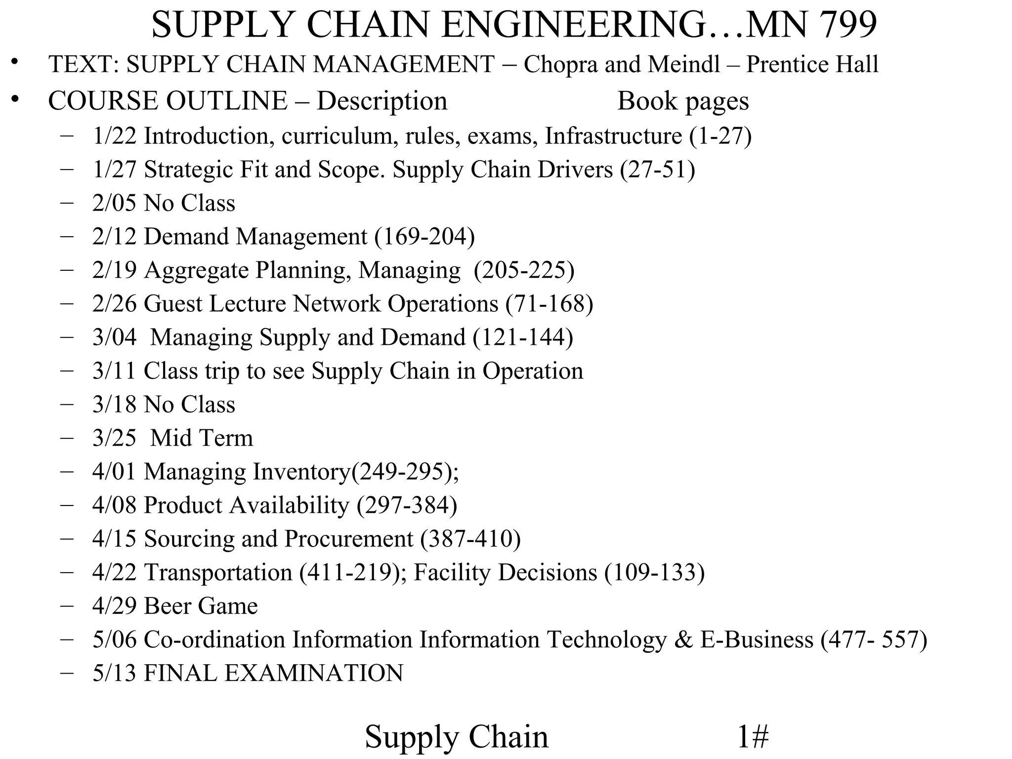
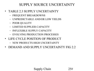
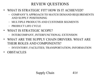
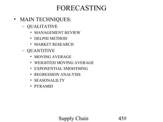
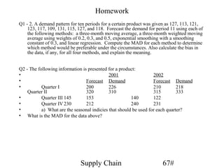
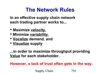
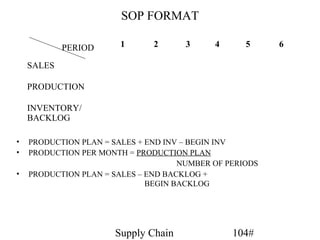
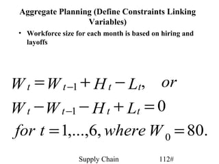
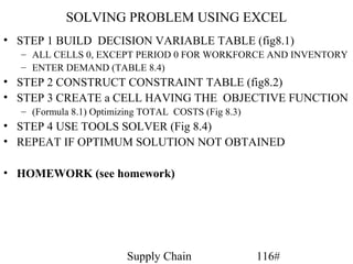
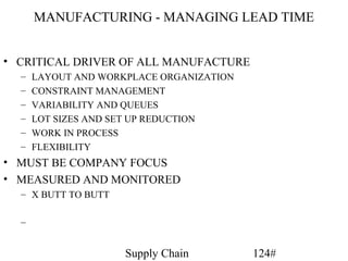
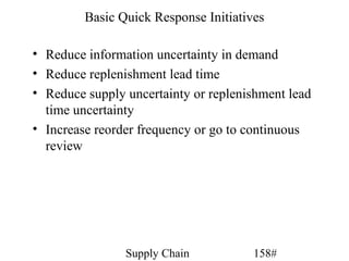
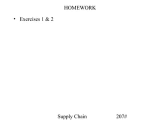
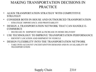
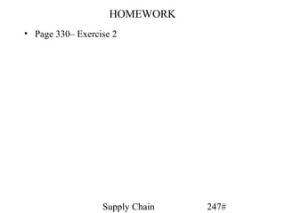
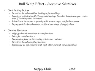
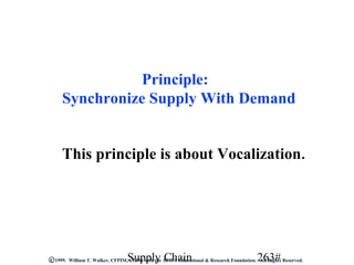
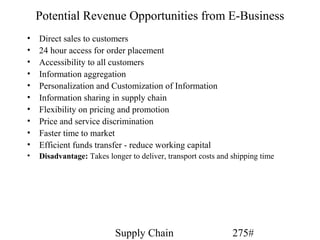
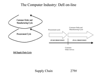
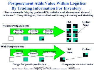
![Simple Trended Series — Example
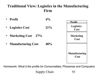
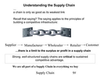
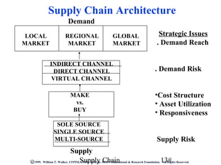
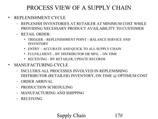
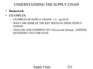
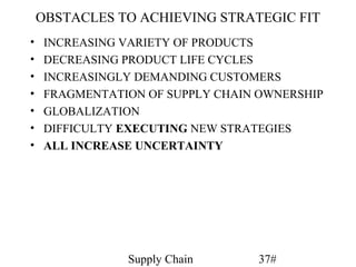
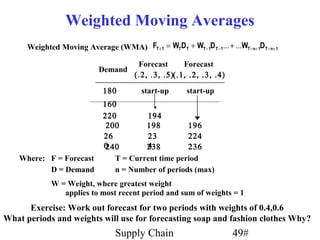
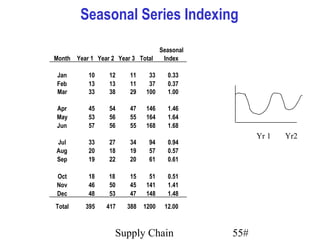
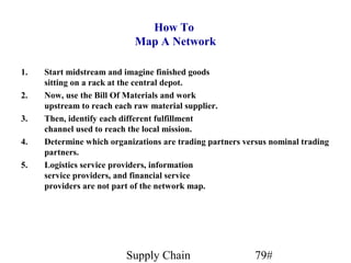
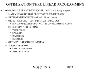
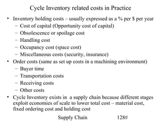
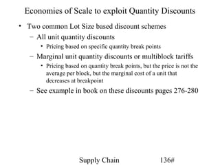
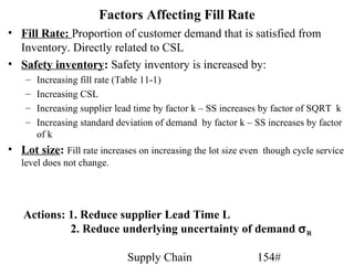
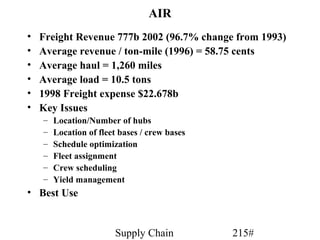
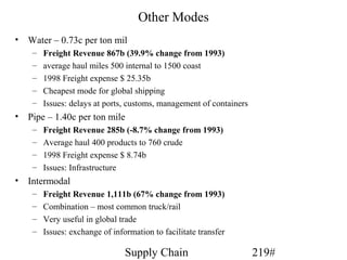
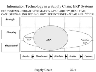
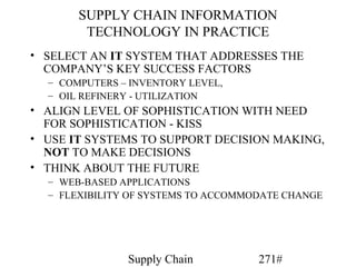
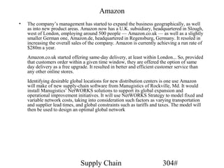
Algebraic Trend Projection
X Y a. Trend (“rise” over “run”) = (13 - 4)/3 = 3 = b
0 4 b.Y-intercept (a) = “compute”
1 7 the Y value for X = 0, thus Y-int = 4
2 10
3 13 c. Period 4: Y = a + bX = 4 + 3 (4 [for period 4]) = 16
13
10
Rise
7
4 Run
1 2 3
Supply Chain 52#](https://image.slidesharecdn.com/poly-supply-chain-engin-mn-799-1213140782078568-8-130219171852-phpapp01/85/Poly-supply-chain-engin-mn-799-1213140782078568-8-52-320.jpg)
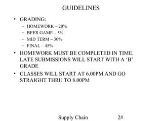
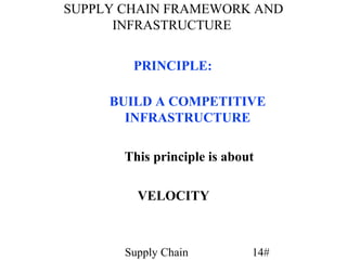
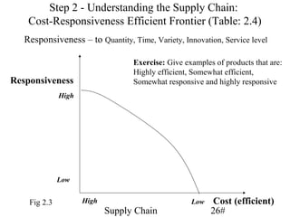
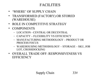
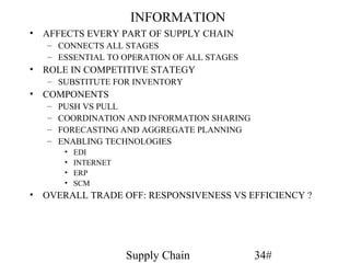
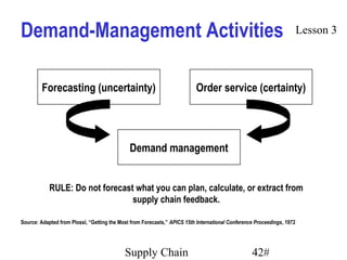
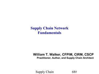
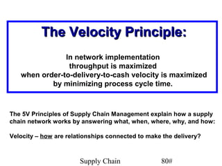
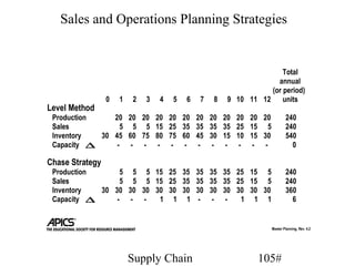
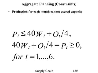
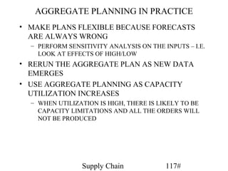
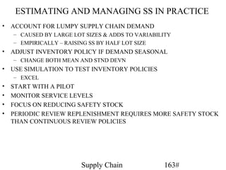
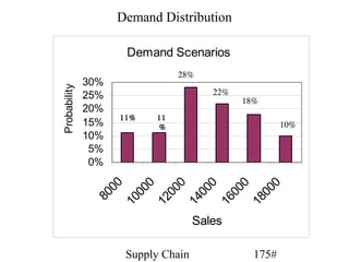
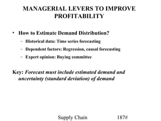
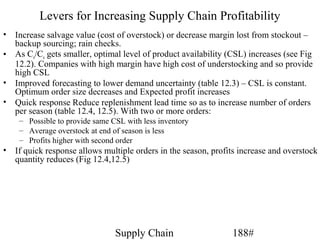
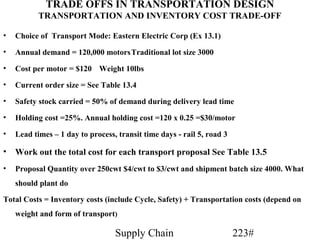
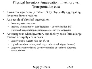
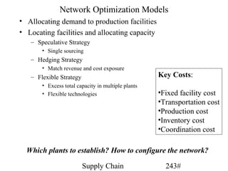
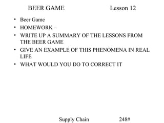
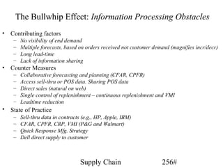
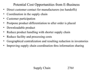
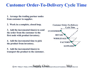
![TRENDED TIME SERIES FORECASTING
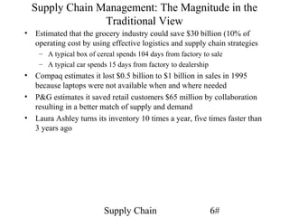
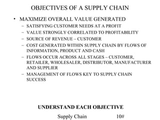
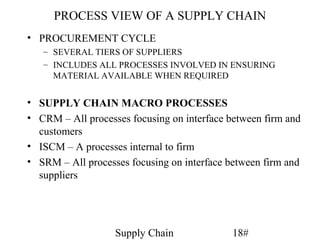
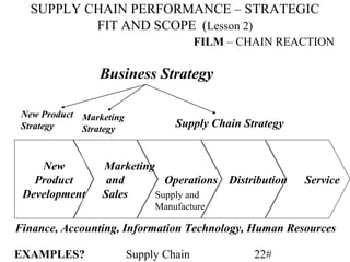
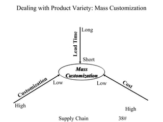
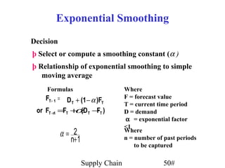
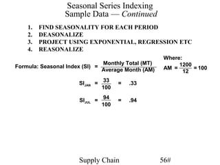
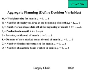
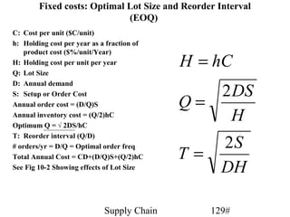
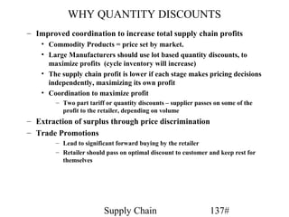
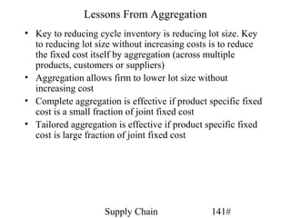
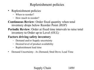
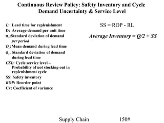
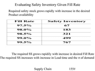
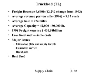
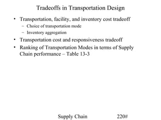
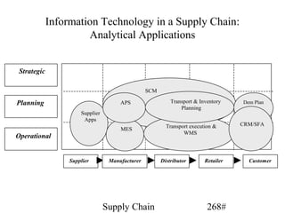
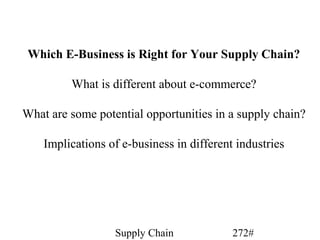
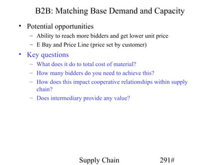
• Question: How do you forecast a seasonal item
• Y(forecast) = [A (intercept) + X (trend) x T (time period) ]
x S (seasonality factor)
• FIRST DETERMINE LEVEL AND TREND - IF SEASONAL
DESEASONALIZE
• THEN FORECAST USING EXPONENTIAL OR TREND
• RESEASONALIZE
Supply Chain 54#](https://image.slidesharecdn.com/poly-supply-chain-engin-mn-799-1213140782078568-8-130219171852-phpapp01/85/Poly-supply-chain-engin-mn-799-1213140782078568-8-54-320.jpg)
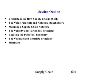
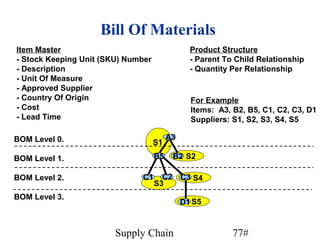
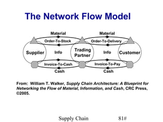
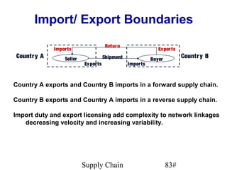
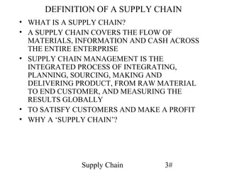
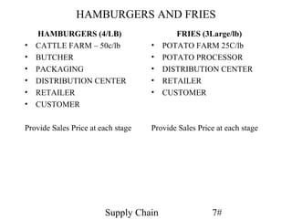
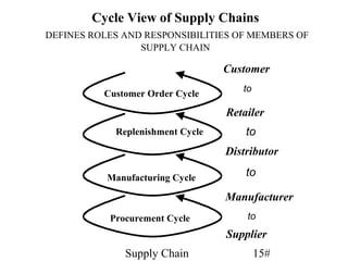
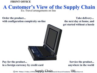
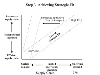
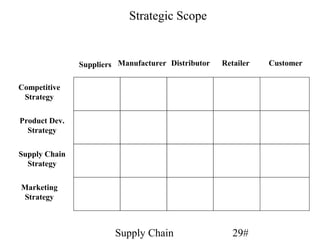
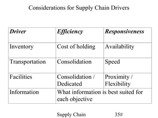
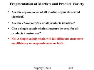
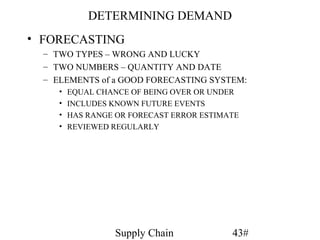
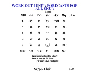
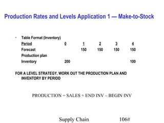
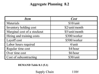
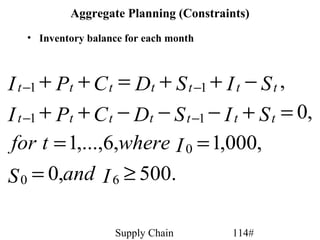
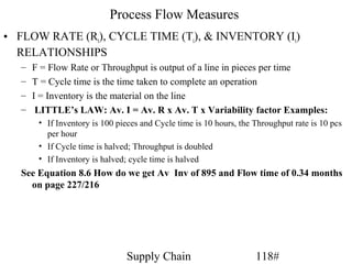
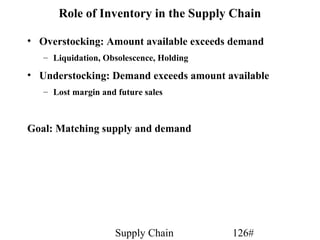
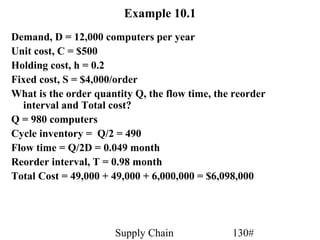
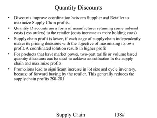
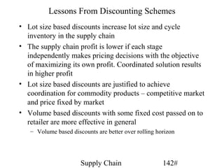
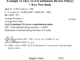
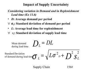
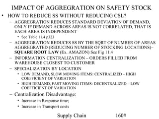
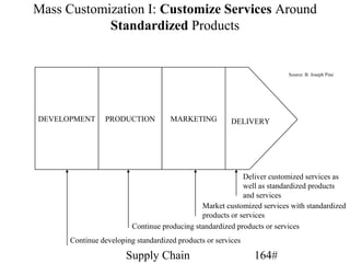
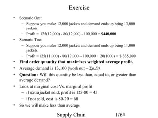
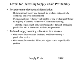
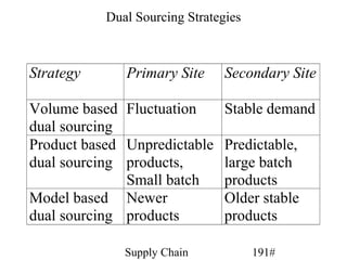
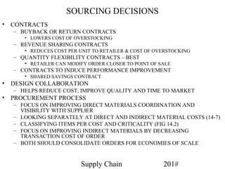
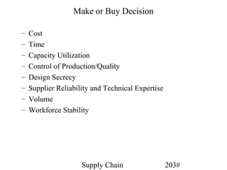
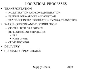
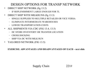
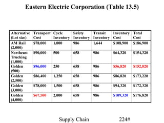
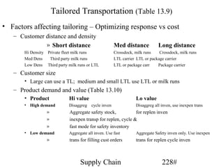
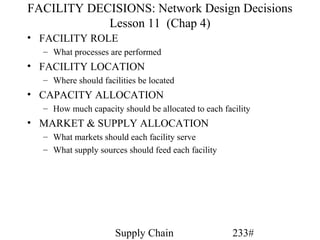
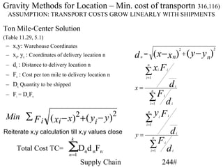
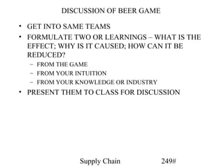
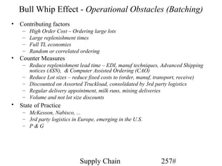
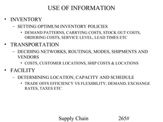
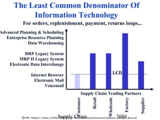
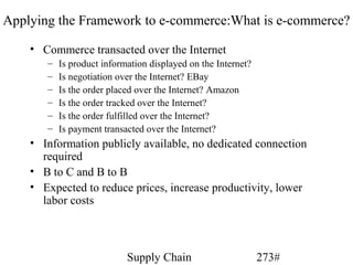
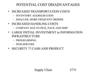
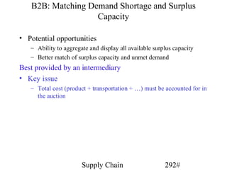
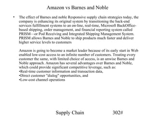
![Packaging And Labeling
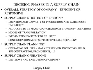
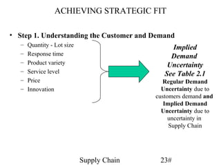
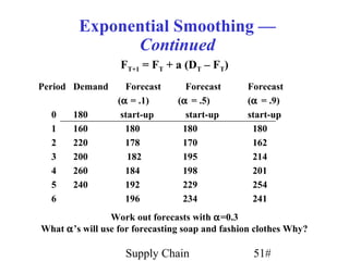
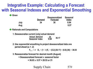
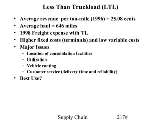
[ ] Cartons, plastic cushions, and labels
Cartons may be missing from the product BOM.
[ ] RFID/ bar code on all packaging.
[ ] Select a wall thickness and box burst
Master strength to protect the product.
Carton
[ ] Keep Country Of Origin labeling consistent
from the product to the outside packaging.
[ ] Transportation and warehousing costs
Unit Load are a function of cubic dimensions and weight.
[ ] Items that have to be repalletized for
transport or storage cost more.
Supply Chain 96#](https://image.slidesharecdn.com/poly-supply-chain-engin-mn-799-1213140782078568-8-130219171852-phpapp01/85/Poly-supply-chain-engin-mn-799-1213140782078568-8-96-320.jpg)
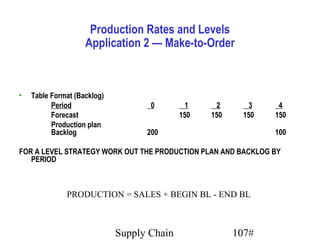
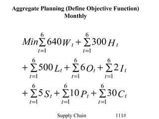
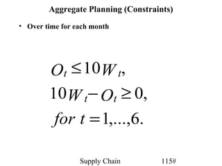
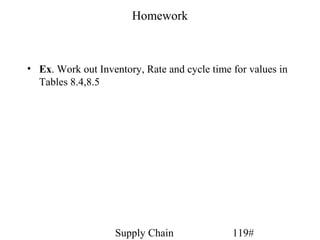
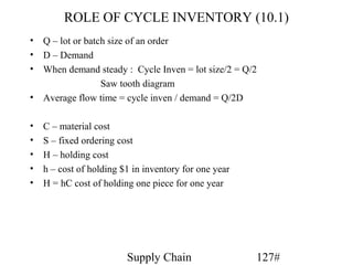
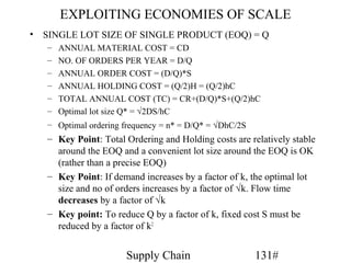
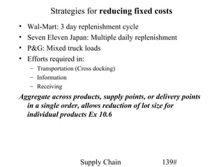

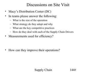
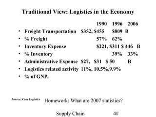
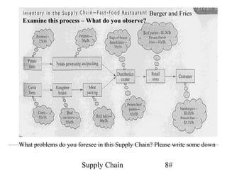
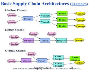
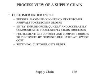
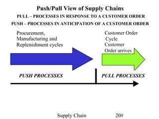
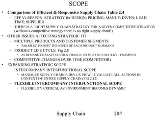
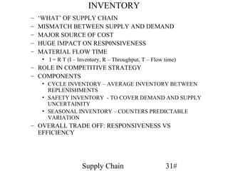
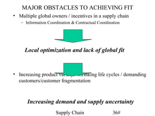
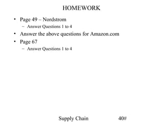
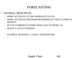
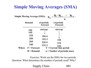
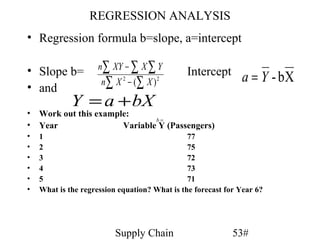
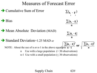
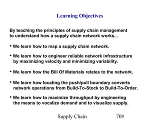
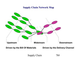
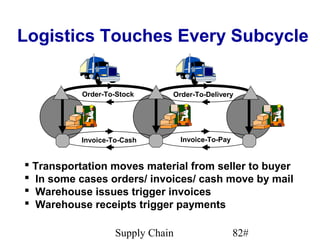
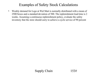
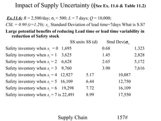
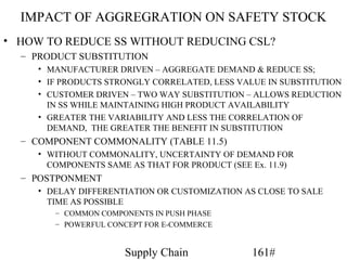
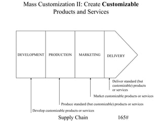
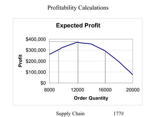
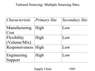
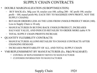
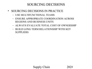
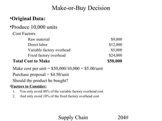
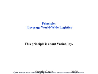
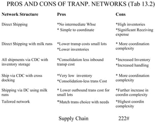
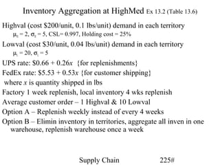
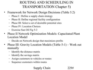
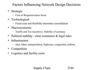
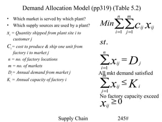
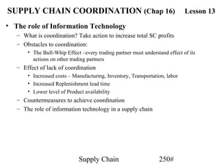
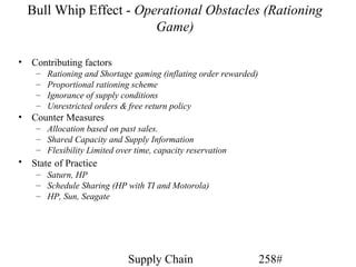
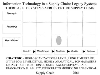
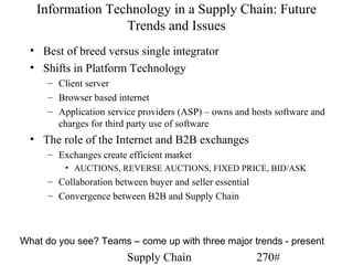
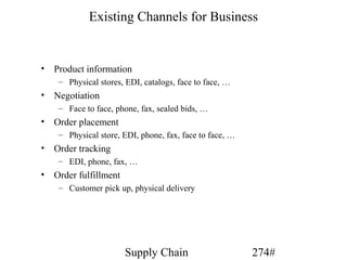
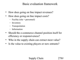
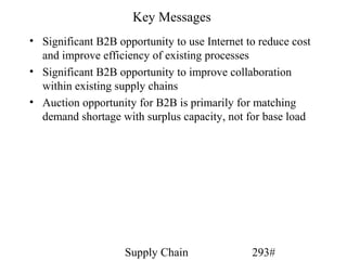
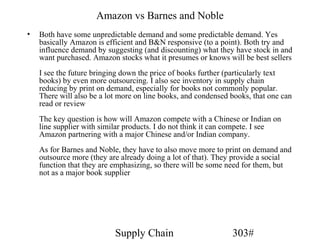
![FORMULAS USED FOR CALCULATING SERVICE LEVELS
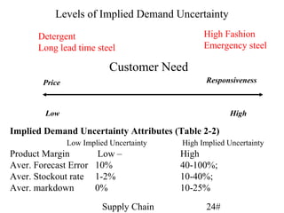
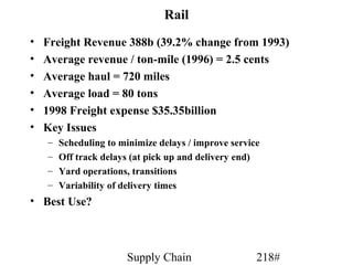
D L
= LD
σ L
= Lσ D
ROP = D L + ss
CSL = F ( ROP, D L ,σ L )
cv = σ / µ
CSL = F ( ROP, DL ,σ L ) = NORMDIST ( ROP, D L ,σ L ,1)
fr = 1 − ESC / Q = (Q − ESC ) / Q
orESC = −( ss[1 − NORMDIST ( ss / σ L ,0,1,1] + σ L NORMDIST ( ss / σ L ,0,1,1)
Supply Chain 151#](https://image.slidesharecdn.com/poly-supply-chain-engin-mn-799-1213140782078568-8-130219171852-phpapp01/85/Poly-supply-chain-engin-mn-799-1213140782078568-8-151-320.jpg)
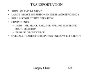
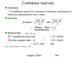
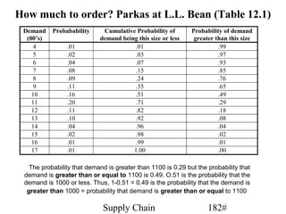
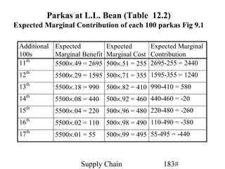
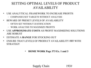
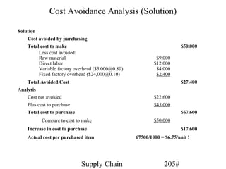
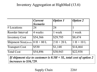
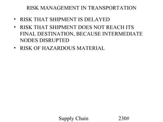
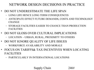
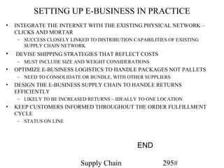
![Parkas at L.L. Bean
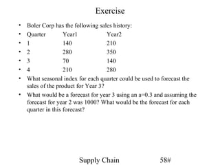
Cost per parka = $45
Sale price per parka = $100
Discount price per parka = $50
Holding and transportation cost = $10
• Profit from selling parka = $100-$45 = $55
• Cost of overstocking = $45+$10-$50 = $5
• Expected demand = =1026, ordered 1000 parkas CSL51%
•
• See formula on page 224
∑
Expected profit from ordering 1000 parkas = $49,900
Di pi
– Expected profit =
10
∑ [ Di ( p − c ) − (1000 − Di )(c − s )] pi + (1 − Pi )1000 ( p − c )
i= 4
Supply Chain 180#](https://image.slidesharecdn.com/poly-supply-chain-engin-mn-799-1213140782078568-8-130219171852-phpapp01/85/Poly-supply-chain-engin-mn-799-1213140782078568-8-180-320.jpg)
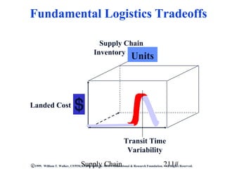
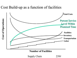


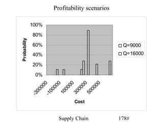
Here are the key points about inventory as a driver of supply chain performance: - Inventory is a major cost but enables responsiveness by bridging mismatches between supply and demand. - The level and placement of inventory impacts efficiency and responsiveness. Higher inventory improves responsiveness at the cost of efficiency. - Inventory levels and management should be aligned with competitive strategy - more inventory is needed for responsive strategies focusing on availability and fill rates. - Common inventory components include cycle inventory to bridge replenishment cycles and safety stock to protect against uncertainties in demand or supply. Managing these components is important to balance costs and customer service. - Information technology can help optimize inventory levels by improving demand forecasting, replenishment processes,


