![ISA Transactions 77 (2018) 146–166
Practice article
Fuzzy logic for plant-wide control of biological wastewater treatment
process including greenhouse gas emissions
I. Santín a,b,*
, M. Barbu a,c
, C. Pedret a
, R. Vilanova a
a
Department of Telecommunications and Systems Engineering, School of Engineering, Universitat Autònoma de Barcelona, 08193, Bellaterra, Barcelona, Spain
b
Escola Universitria Salesiana de Sarrià, Passeig Sant Joan Bosco 74, 08017 Barcelona, Spain
c Department of Automatic Control and Electrical Engineering, “Dunarea de Jos” University of Galati, 800008 Galati, Romania
a r t i c l e i n f o a b s t r a c t
Article history:
Received 20 November 2017
Revised 9 April 2018
Accepted 13 April 2018
Available online 25 April 2018
Keywords:
Fuzzy control
Wastewater treatment plants
GHGemissions
Benchmark simulation model no 2 gas
The application of control strategies is increasingly used in wastewater treatment plants with the aim of
improving effl uent quality and reducing operating costs. Due to concerns about the progressive growth of
greenhouse gas emissions (GHG), these are also currently being evaluated in wastewater treatment plants.
The present article proposes a fuzzy controller for plant-wide control of the biological wastewater treatment
process. Its design is based on 14 inputs and 6 outputs in order to reduce GHG emissions, nutrient concentra-
tion in the effl uent and operational costs. The article explains and shows the effect of each one of the inputs
and outputs of the fuzzy controller, as well as the relationship between them. Benchmark Simulation Model
no 2 Gas is used for testing the proposed control strategy. The results of simulation results show that the
fuzzy controller is able to reduce GHG emissions while improving, at the same time, the common criteria of
effl uent quality and operation al costs.
© 2018 ISA. Published by Elsevier Ltd. All rights reserved.
1. Introduction
Wastewater treatment plants (WWTPs) are used worldwide to
ensure the suitable water quality for the receiving environment.
Some of the pollutants are reduced to allowed levels by the default
WWTP structure without applying any automatic control. However,
other pollutants are more diffi cult to be reduced. For this reason and
also to restrict operational costs, the application of control engineer-
ing in WWTPs is playing an important role in research in recent years
(Vilanova et al. [1,2]).
Another major issue regarding to WWTPs is the greenhouse gas
(GHG) emissions generated during the treatment process. Actually,
GHG emissions are important in maintaining the proper tempera-
ture for life on Earth, since they retain part of the infrared radiations
reflected from the surface of the Earth. The problem is that the GHG
emissions increase generated by the industrialized world is creating
a global climate change, which can cause serious impacts on both the
land and socioeconomic systems.
* Corresponding author. Department of Telecommunications and Systems Engi-
neering, School of Engineering, Universitat Autònoma de Barcelona, 08193, Bellaterra,
Barcelona, Spain.
E-mail addresses: Ignacio.Santin@uab.cat (I. Santín), Marian.Barbu@ugal.ro (M.
Barbu), Carles.Pedret@uab.cat (C. Pedret), Ramon.Vilanova@uab.cat (R. Vilanova).
Among the GHG emitted in the wastewater treatment process,
the present paper focus on the nitrous oxide (N2O) emissions dur-
ing the nitrification process, on the carbon dioxide (CO2) emissions
due to endogenous respiration of biomass, on CO2 generated from
external carbon source production and on CO2 due to electric con-
sumption.
There are previous works in the literature as Kimochi et al. [3],
Kampschreur et al. [4], Foley et al. [5], Law et al. [6], Flores-Alsina
et al. [7,8], Aboobakar et al. [9] or Wang et al. [10], which show that
N2O is an intermediate in the nitrification of WWTPs and that it has a
high impact in the GHG emissions. Incomplete nitrification or deni-
trification can lead to an accumulation of nitrite concentration (SNO2
)
that triggers the production of N2O emissions. The endogenous res-
piration of the biomass is a process of autoxidation that takes place
after the depletion of food reserves. In this process, the microorgan-
isms metabolize their own cellular material until its own destruction
generating CO2 emissions, as explained in Monteith et al. [11]. In the
case of the electric consumption, it is related to the fact that the elec-
tricity is mostly generated by burning fossil fuels, which generates
CO2 emissions.
In this article, the control strategies applied to cope with effl uent
quality, costs and GHG emissions have been tested using the Bench-
mark Simulation Model no 2 Gas (BSM2G), which was introduced
by Flores-Alsina et al. [7]. This benchmark has been modified over
the last years by the same authors, who added ammonia oxidizing
https://doi.org/10.1016/j.isatra.2018.04.006
0019-0578/© 2018 ISA. Published by Elsevier Ltd. All rights reserved.
Contents lists available at ScienceDirect
ISA Transactions
journal homep ag e: www. elsevi er. com/locat e/isat rans](https://image.slidesharecdn.com/fuzzy-logic-for-plant-wide-control-of-biological-wastewater-tr2018isa-tran-191011175840/75/Fuzzy-logic-for-plant-wide-control-of-biological-wastewater-treatment-process-including-greenhouse-gas-emissions-1-2048.jpg)
![I. Santín et al. / ISA Transactions 77 (2018)146–166 147
List of abbreviations
AE Aeration Energy (kWh/d)
AOB Ammonia Oxidizing Bacteria
ASM1 Activated Sludge Model no. 1
BOD5 5-day Biological Oxygen Demand (mg/l)
Qa Internal recycle flow rate (m3
/d)
qEC External carbon flow rate (m3
/d)
Qin Influent flow rate (m3
/d)
qEC,1 External carbon flow rate in the first tank (m3
/d)
Qw Wastage flow rate (m3
/d)
Qst Flow rate from the storage tank (m3
/d)
BSM1 Benchmark Simulation Model no 1 SNtot Total nitrogen concentration (mg/l)
BSM2 Benchmark Simulation Model no 2
BSM2G Benchmark Simulation Model no 2 Gas
CO2 Carbon dioxide (kg/d)
COD Chemical Oxygen Demand (mg/l)
CODt total Chemical Oxygen Demand (mg/l)
DCS Default COntrol Strategy
EC External Carbon (kg/d)
EQI Effl uent Quality Index (kg of pollutants/d)
GHG Greenhouse gases
HEnet Net Heating Energy (kWh/d)
SNtot,e
Total nitrogen concentration in the effl uent (mg/l)
SNH Ammonium and ammonia nitrogen concentration
(mg/l)
SNH,in Ammonium and ammonia nitrogen concentration at
the input of the primary clarifier (mg/l)
SNH,i Ammonium and ammonia nitrogen concentration in
tank i (mg/l)
SNH,e Ammonium and ammonia nitrogen concentration in
the effl uent (mg/l)
SNO Nitric Oxide concentration (mg/l)
HRT Hydraulic Retention Time (s)
KL a Oxygen transfer coeffi cient (d−1
)
KLai Oxygen transfer coeffi cient in tank i (d−1
)
ME Mixing Energy (kWh/d)
METprod Methane production in the anaerobic digester (kg/d)
N2O Nitrous oxide (kg equivalent CO2/d)
SNO2
SNO3
SNO3 i
SNKj
SN2O
Nitrite concentration (mg/l)
Nitrate concentration (mg/l)
Nitrate concentration in tank i (mg/l)
Kjeldahl nitrogen (mg/l)
Dissolved nitrous oxide concentration (mg/l)
SO Dissolved oxygen concentration (mg/l)
N2 dinitrogen CO2/d)
OCI Overall Cost Index
SO,i Dissolved oxygen concentration in tank i (mg/l)
SP Sludge Production (kg/d)
PE Pumping Energy (kWh/d)
PI Proportional-Integral
Tas Temperature (◦C)
Q Flow rate (m3
/d)
TSS Total Suspended Solids (mg/l)
WWTP Wastewater Treatment Plants
bacteria (AOB) denitrification pathway for N2O emissions based on
Guo and Vanrolleghem [12]. In addition, BSM2G is the result of the
evolution of previous benchmarks. First, the Benchmark Simulation
Model no 1 (BSM1) was developed in Copp [13], which includes
the biological treatment and a secondary clarifier, using one-week
period to evaluate results. Next, the Benchmark Simulation Model no
2 (BSM2) (Gernaey et al. [14]) included the whole cycle of a WWTP,
adding the sludge treatment and a primary clarifier, applying a more
complete influent with a one-year period for evaluation. BSM2G dif-
fers from BSM2 mainly in the inclusion of GHG emissions assess-
ment. It should be noted that the use of models for the evaluation of
GHG emissions is currently restricted to the research domain, due to
the incomplete knowledge regarding the SNO2
production pathways
(Mannina et al. [15], Ni and Yuan [16]).
Although the present work uses Proportional-Integral (PI) con-
trollers, the main contribution is based on a fuzzy controller to cope
with the mentioned problems in WWTPs. There are already many
works in the literature that have applied fuzzy control strategies
in WWTPs. For example, the fuzzy controller was applied for the
basic control loop of the dissolved oxygen concentration (SO) in the
fifth reactor (SO,5) by using BSM1 in Belchior et al. [17] and Nasr
et al. [18] or in a pilot plant in Traore et al. [19]. In the case of
Santín et al. [20] and Meyer and Pöpel [21], the fuzzy controller is
used for ammonium and ammonia nitrogen concentration (SNH) in
the fifth tank (SNH,5) cascade control by manipulating the SO,5 set-
point, also by using BSM1 as testing plant. The fuzzy inference sys-
tem is employed in Pai et al. [22] to improve artificial neural net-
work to predict the total suspended solids (TSS) and the chemi-
cal oxygen demand (COD) in the effl uent from a hospital WWTP.
By using BSM2 as a working scenario, Santín et al. [23] Santín et
al. [24] apply fuzzy control to deal with pollutants limits viola-
tions. Fuzzy logic has also been applied for evaluation (Kalavrouzi-
otis et al. [25]) or management (Hirsch et al. [26]) of real WWTPs.
However, none of the referred papers have taken into account GHG
emissions.
Although there is a large number of works that apply control
strategies in WWTPs, the evaluation of GHG emissions has emerged
in recent years. Some works that analyze GHG emissions in WWTPs
by applying control strategies are Flores-Alsina et al. [7,8] and Barbu
et al. [27]. They use BSM2G, but with different model versions.
Flores-Alsina et al. [7] tests the effect of traditional control strate-
gies in GHG emissions, but without considering those produced by
nitrification. Flores-Alsina et al. [8] shows the effect on GHG emis-
sions of the different areas of a WWTP. Barbu et al. [27] presents the
effects of other traditional control strategies on water quality, opera-
tional costs and, especially, on GHG emissions, by an integral indica-
tor for performance evaluation. However, it was not the goal of these
works to implement specific control strategies in order to reduce N2O
emission in the nitrification process. On the other hand, Santín et
al. [28] reduce N2O emissions combining cascade SNO2
control and
cascade SNH,5 control. Boiocchi et al. [29] reduce N2O emissions with
a fuzzy controller that manipulates the oxygen transfer coeffi cient
(KLa) of the aerobic reactors based on SNH and the nitrate concen-
tration (SNO3
) in the input and in the output of the nitrification pro-
cess. In addition, Boiocchi et al. [29] take into account the effect that
the oxygen aeration can produce on effl uent costs and quality. Santín
et al. [28] combine two control strategies with PI controllers to also
reduce costs and improve the effl uent quality, but without attempt-
ing to eliminate nutrient violations. Both articles only manipulate
KLa of the aerobic reactors and only reduce SNO2
as GHG emissions.
The present article reduces the SNO2
emissions using a different
control strategy than the two referred articles, by means of only](https://image.slidesharecdn.com/fuzzy-logic-for-plant-wide-control-of-biological-wastewater-tr2018isa-tran-191011175840/75/Fuzzy-logic-for-plant-wide-control-of-biological-wastewater-treatment-process-including-greenhouse-gas-emissions-2-2048.jpg)
![148 I. Santín et al. / ISA Transactions 77 (2018)146–166
Fig. 1. BSM2 plant with notation used for flow rates.
SNH sensors, which are commonly used in real plants. The proposed
controller not only manipulates SO in the third reactor (SO,3), SO in
the fourth reactor (SO,4) and the SO,5 set-points, but also the inter-
nal recirculation flow rate (Qa), the external carbon flow rate (qEC)
in the first reactor (qEC,1) and the flow rate from the storage tank
(Qst). This fact also allows the proposed paper to differentiate itself
from the mentioned referenced articles, by reducing the CO2 emis-
sions due to the endogenous respiration of biomass, CO2 generated
from the external carbon source production and CO2 due to the elec-
tric consumption, and by removing the limit violations of the nutri-
ents. The proposed control strategies also differ from the literature,
achieving these objectives (together with the reduction of costs) by
the implementation of a single fuzzy controller, which to the best
of the authors knowledge has not been previously proposed. Also, it
has to be emphasized the addition of the derivatives of some vari-
ables with respect to time as fuzzy controller inputs, in order to
act in advance. In addition, the temperature is also considered as a
fuzzy controller input, since higher temperature means higher GHG
emissions (Boiocchi et al. [29]) and lower temperature means more
total nitrogen concentration (SNtot
) and SNH are generated. The article
explains the contribution of each manipulated variable in the pro-
posed objectives, as well as the effects of each of the fuzzy controller
al. [14]) that includes GHG emissions. The model was presented in
Flores-Alsina et al. [7] and an updated version provided by the same
authors has been used for the present article. Within these modifica-
tions, it is included the incorporation of the AOB denitrification path-
way for N2O emissions based on Guo and Vanrolleghem [12]. There-
fore, the present BSM2G includes two pathways for N2O emissions
(heterotrophic denitrification and AOB denitrification).
2.1. Layout
The BSM2G layout (Fig. 1) is designed for an influent with an aver-
age flow rate of 20,648.36 m3
/d and an average biodegradable COD of
592.53 mg/l. In the same way as in the case of BSM2, BSM2G is made
up of a primary clarifier, a secondary treatment and a sludge treat-
ment. The secondary treatment includes the biological reactors and
a secondary settler.
For the biological treatment, BSM2G includes, as in BSM1 (Copp
[13]) and BSM2, five biological reactors, two of which are anoxic
and three are aerobic. The biological reactions inside the reactors are
modeled by the Activated Sludge Model no 1 (ASM1) (Henze et al.
[30]). In BSM2G, ASM1 is extended on the basis of Hiatt and Grady
[31] and Mampaey et al. [32] in order to include, besides SNO , the
input. It should be noted that the proposed fuzzy control looks for a 3
other compounds that are present in the nitrification and deni tri-
trade-off between the aforementioned objectives, achieving satisfac- fication processes: SNO , nitric oxide (SNO), N2O and dinitrogen (N2).
tory results and without meaningfully worsening any of them. 2There is an internal r tion from the last aerobic reactor to feed
The paper is organized as follows. First, BSM2G working scenario
is presented. Next, the default and the proposed control strategies
are explained. Afterwards, simulations results are shown, together
with the discussion about them. Finally, the most important conclu-
sions are drawn.
2. Materials and methods
A benchmark is used for the evaluation of the proposed con-
trol strategy, as it is a common practice in wastewater treatment
research. This is BSM2G, which is an extension of BSM2 (Gernaey et
ecircula
the first anoxic reactor with SNO3
. The secondary clarifier is mod-
eled as a 10 layers non-reactive unit. At lower levels the sludge is
deposited by gravity. Some of this sludge is recirculated to the first
anoxic reactor (external recirculation) and the other part is led to be
treated. The hydraulic retention time of the primary clarifier and the
secondary treatment is 22 h. It is based on the average dry weather
flow rate and the volume of the primary clarifier (900 m3
), the bio-
logical reactors (12,000 m3
) and the secondary settler (6000 m3
). The
volume of each of the two anoxic tanks is 1500 m3
and the volume
of each of the three aerobic tanks is 3000 m3
.](https://image.slidesharecdn.com/fuzzy-logic-for-plant-wide-control-of-biological-wastewater-tr2018isa-tran-191011175840/75/Fuzzy-logic-for-plant-wide-control-of-biological-wastewater-treatment-process-including-greenhouse-gas-emissions-3-2048.jpg)
![I. Santín et al. / ISA Transactions 77 (2018)146–166 149
Table1
Limits for the effl uent pollutants.
Variable Value
SNtot
<18 mg/l
CODt <100 mg/l
SNH <4 mg/l
TSS <30 mg/l
BOD5 <10 mg/l
For the sludge treatment, BSM2G makes use of a thickener, an
anaerobic digester and a dewatering unit. The water extracted from
the sludge by the dewatering process is recirculated to the primary
clarifier through the storage tank to regulate its flow rate.
The influent data in BSM2G includes rainfall and storm events, as
well as variations in temperature. It is defined for 609 days, but only
the results of the period from day 245 to day 609 are considered for
evaluation. With the aim to stabilize the plant, a constant influent is
applied to the plant for 200 days, before any simulation.
2.2. Evaluation criteria
The performance of the control strategies is evaluated by consid-
ering the effl uent quality, the operational costs and the GHG emis-
sions.
The evaluation criteria for the effl uent quality are the percentage
of time for which the values of the effl uent pollutants are over the
established limits and the Effl uent Quality Index (EQI). Table 1 shows
the limits established for the effl uent concentrations of SNtot
, total
COD (CODt), SNH, TSS and 5-day Biological Oxygen Demand (BOD5) In
BSM2G, SNtot
is the sum of SNO3
, SNO2
, SNO, SN2O
and Kjeldahl nitrogen
(SNKj), which includes the organic nitrogen and SNH. Within these
concentrations, this article only evaluates the violations of SNtot
in
the effl uent (SNtot,e
) and SNH in the effl uent (SNH,e). This is due to the
fact that the rest of the concentrations are commonly kept under the
established limits and they only exceed the limits in exceptional days
when the high increase of the influent flow makes the wastewater be
bypassed to the effl uent without being treated.
EQI is expressed in Kg of pollutants per day and is calculated
weighting the effl uent concentration of the different pollutants,
according to the following expression:
t=609days
treatment, the sludge treatment, the difference between electric con-
sumption and electric generation, the EC production and the sludge
to be disposed. Within these sources, with the control strategy pro-
posed in this article, those produced in the biological treatment, due
to electricity and due to EC production are attempted to be reduced
and then evaluated.
3. Control approach
The control approach proposed in this article is mainly based on
a single fuzzy controller that manipulates the variables of the water
line in a WWTP. However, although the work is focused on this fuzzy
controller, three PI controllers are also applied in order to control
SO,3, SO,4 and SO,5 by manipulating KLa in the third tank (KLa3), in
the fourth tank (KLa4) and in the fifth tank (KLa5). Each one of them
controls the SO of one reactor by manipulating the KLa of the same
reactor.
Due to the large number of inputs and outputs of the pro-
posed fuzzy controller, it has been elaborated incrementally in order
to observe the effect produced by the different manipulated and
measured variables. The fuzzy controller finally designed is called
fuzzy_plantwide and the intermediate fuzzy controllers are num-
bered from 1 to 4 (fuzzy_1, fuzzy_2, fuzzy_3 and fuzzy_4).
In order to compare the performance of the new proposals, the
default control strategy (DCS) used in BSM2G is considered the start-
ing point. The second part includes the explanations of the PI con-
trollers used at the basic level and the fuzzy controller. Fig. 2 shows
the configuration of DCS and the proposed control strategy.
For all the control strategies, ideal sensors have been considered,
as it is a common practice in the research made on benchmark sim-
ulation models.
3.1. Default control strategy (DCS)
As it is shown in Fig. 2a, the DCS closed-loop control configuration
consists of a PI controller that controls SO,4 at a set-point of 2 mg/l by
manipulating KL a3, KLa4 and KL a5 with KLa5 set to the half value of
KLa3 and KLa4. KL a values are constrained from 0 to 360 d−1
.
For other possible manipulated variables, a fixed value is applied.
qEC,1 is added at a constant flow rate of 2 m3
/d. For the rest of the
reactors there is no external carbon addition. Two different wastage
flow rate (Qw ) values are imposed depending on the time of the year:
from 0 to 180 days and from 364 to 454 days Qw is set to 300 m3
/d;
and for the remaining time periods Qw is set to 450 m3/d. Qa is fixed
EQI =
1
1000 · T ∫
t=245days
(2 · TSS(t) + COD(t) + 30 · SNKj(t)) + at 61,944 m3/d.
The tuning parameters of the PI controller implemented in DCS
are kp = 25 and Ti = 0.002. The tuning employed here is taken from
+ 10 · (SNO3
+ SNO2
+ SNO + SN2O
)(t) + 2 · BOD5(t)) · Q(t) · dt
(1)
Nopens et al. [33] in order to consider the same basic control loops
configuration as in the BSM2 default control strategy.
where T is the evaluation period and Q is the flow rate.
The operational costs are evaluated by the Operational Cost Index
(OCI). It is calculated weighting the different costs of a WWTP as fol-
lows:
OCI = AE + PE + 3 · SP + 3 · EC + ME − 6 · METprod + HEnet (2)
where AE is the aeration energy (kWh/d), PE is the pumping energy
(kWh/d), SP is the sludge production (kg/d), EC refers to the carbon
that could be added to improve denitrification (kg/d), ME is the mix-
ing energy (kWh/d), METprod is the produced methane (kWh/d) and
HE is the heating energy (kWh/d).
The GHG emissions are a new evaluation criterion of BSM2G with
respect to BSM2. They are calculated according to the principles pro-
posed by Hiatt and Grady [31] and Mampaey et al. [32]. The follow-
ing sources of GHG emissions are taken into account: the biological
3.2. Proposed control strategy
The proposed control strategy in this paper is mainly focused on
the implementation of fuzzy logic. The own authors’ experience in
WWTP control engineering and the opinions received from opera-
tors in real plants make the authors conclude that the experience
and knowledge of the plant behavior is of great importance in the
control strategies application in WWTPs. For this reason, the main
control proposed is based on a single fuzzy controller designed to
manipulate six variables of the water line based on different mea-
sured variables, as well as their time derivatives in some cases, to
know their trend over time. The fuzzy controller does not try to keep](https://image.slidesharecdn.com/fuzzy-logic-for-plant-wide-control-of-biological-wastewater-tr2018isa-tran-191011175840/75/Fuzzy-logic-for-plant-wide-control-of-biological-wastewater-treatment-process-including-greenhouse-gas-emissions-4-2048.jpg)
![150 I. Santín et al. / ISA Transactions 77 (2018)146–166
the measured variables at a given set-point, as in Santín et al. [20].
The configuration of the full proposed control strategy is shown in
Fig. 2b.
Within the manipulated variables of the fuzzy controller, Qa, qEC,1
and Qst are directly related to the actuator. However, SO in the
aerobic reactors are controlled by PI controllers, whose set-points
are manipulated by the fuzzy controller. These PI controllers are
explained in the next section.
3.2.1. PI controllers for SO control in the aerobic reactors
PI controllers aim to maintain a variable at a given set-point
(unlike the proposed fuzzy controller) and they are mostly used in
real plants. SO in the reactors are some of the few variables that can
be maintained at a set-point in a WWTP, without a large error. There-
fore, PI controllers are proposed for this objective. For the fuzzy logic,
it is easier and more coherent to find the relationship of SNH and SNO3
with SO in the aerobic reactors, than directly with KL a of the aerobic
reactors.
The tuning of these PI controllers as well as the controlled and
manipulated variables of each one are the same with those the
default PI controller (kp = 25 and Ti = 0.002). This is because their
tracking is satisfactory enough and the implementation objectives of
this article are focused on the fuzzy controller. KLa values are also
constrained from 0 to 360 d−1
as in DCS.
3.2.2. Fuzzy logic
Fuzzy logic can be defined as a control based on human exper-
tise, determined by words instead of numbers and sentences instead
of equations. However, process variables are measured in numbers
instead of words. For this reason, the fuzzy controller adapts the
input variables into suitable linguistic values by membership func-
tions (mf). For further information about the fuzzy control, the reader
is referred to standard references such as Klir and Yuan [34].
The proposed fuzzy controller has been initially tuned based on
the knowledge of the biological processes described by the extended
ASM1 and on a specific analysis of the evolution over time of the
fuzzy controller inputs. After that, the membership functions values
range have been adjusted by trial and error in order to optimize the
results. The proposed fuzzy controller has been designed and tested
progressively. It has been always implemented with a sampling time
of 15 min. The complete fuzzy controller is called fuzzy_plantwide,
which consists of 14 inputs, 6 outputs, and 80 fuzzy rules. For the
controller inputs, 8 sensors are required. As shown in Figs. 2b and
3, the fuzzy_plantwide inputs are SNH at the input of the biological
reactors (SNH,0), at the output of the second reactor (SNH,2), of the
third reactor (SNH,3), of the fourth reactor (SNH,4) and SNH,5, the sum
of SNO3
at the output of the fifth reactor (SNO3 5) and SNH,5, the tem-
perature (Tas), the input flow rate (Qin ), the product of Qin and SNH
at the input of the primary clarifier (SNH,in), as well as the deriva-
tive with respect to time of SNH,2 (dSNH,2/dt), SNH,3 (dSNH,3/dt), SNH,4
(dSNH,4/dt), the sum of SNH,5 and SNO3 5 (d(SNH,5+SNO3 5)/dt) and the
product of Qin and SNH,in (d(Qin·SNH,in )/dt). The fuzzy_plantwide out-
puts are the SO,3 set-point, the SO,4 set-point, the SO,5 set-point, Qa,
qEC,1 and Qst . Mamdani (Mamdani [35]) is the method of inference.
Fig. 4 shows the most relevant input-output relationships of the
fuzzy controller through surface graphs, which allows the observa-
tion of the non-linearity of the fuzzy controller. The regulation of the
fuzzy controller output variables is aimed to reduce GHG emissions,
to reduce costs and to improve the effl uent quality by reducing SNH,e
and SNtot,e
limit violations. However, the manipulation of each vari-
able has different objectives and there is no variable that tries to ful-
fill all the objectives only by itself. The value of the output variables
is obtained based on the input variables, by means of the so-called
fuzzy rules.
Fig. 2. Layouts ofDCS and fuzzy_plantwide.](https://image.slidesharecdn.com/fuzzy-logic-for-plant-wide-control-of-biological-wastewater-tr2018isa-tran-191011175840/75/Fuzzy-logic-for-plant-wide-control-of-biological-wastewater-treatment-process-including-greenhouse-gas-emissions-5-2048.jpg)
![I. Santín et al. / ISA Transactions 77 (2018)146–166 151
Fig. 3. Inputs and outputs offuzzy_1, fuzzy_2, fuzzy_3, fuzzy_4 and fuzzy_plantwide.
The 80 fuzzy rules relate the manipulated variables to the val-
ues of the measured variables. These input-output relationships are
based on the biological processes that take place during the wastew-
ater treatment, as well as on the plant operation experience. The rea-
sons for the choice of input-output relationships are explained in the
following paragraphs, for each one of the fuzzy controllers. The fuzzy
rules code is presented in appendix A and explained by a scheme in
appendix B. The FIS1
Editor from Matlab, used for the implementa-
tion of the fuzzy controllers, has some constrains in applying differ-
ent conditions. This fact requires the definition of a big number of
fuzzy rules that could be significantly reduced with a more flexible
tool.
In order to know the effect produced in the plant by the differ-
ent inputs and outputs, the controller has been tested and explained
incrementally by different steps until the fuzzy_plantwide has been
implemented. To this end, the fuzzy controllers have been numbered
from 1 to 4, as inputs and/or outputs have been added. Fig. 3 show
the inputs and outputs of each of these fuzzy controllers. The code
of fuzzy_plantwide is shown in Appendix A. The objectives sought in
each of the fuzzy controllers, as well as the reasons for their applica-
tion, are explained below.
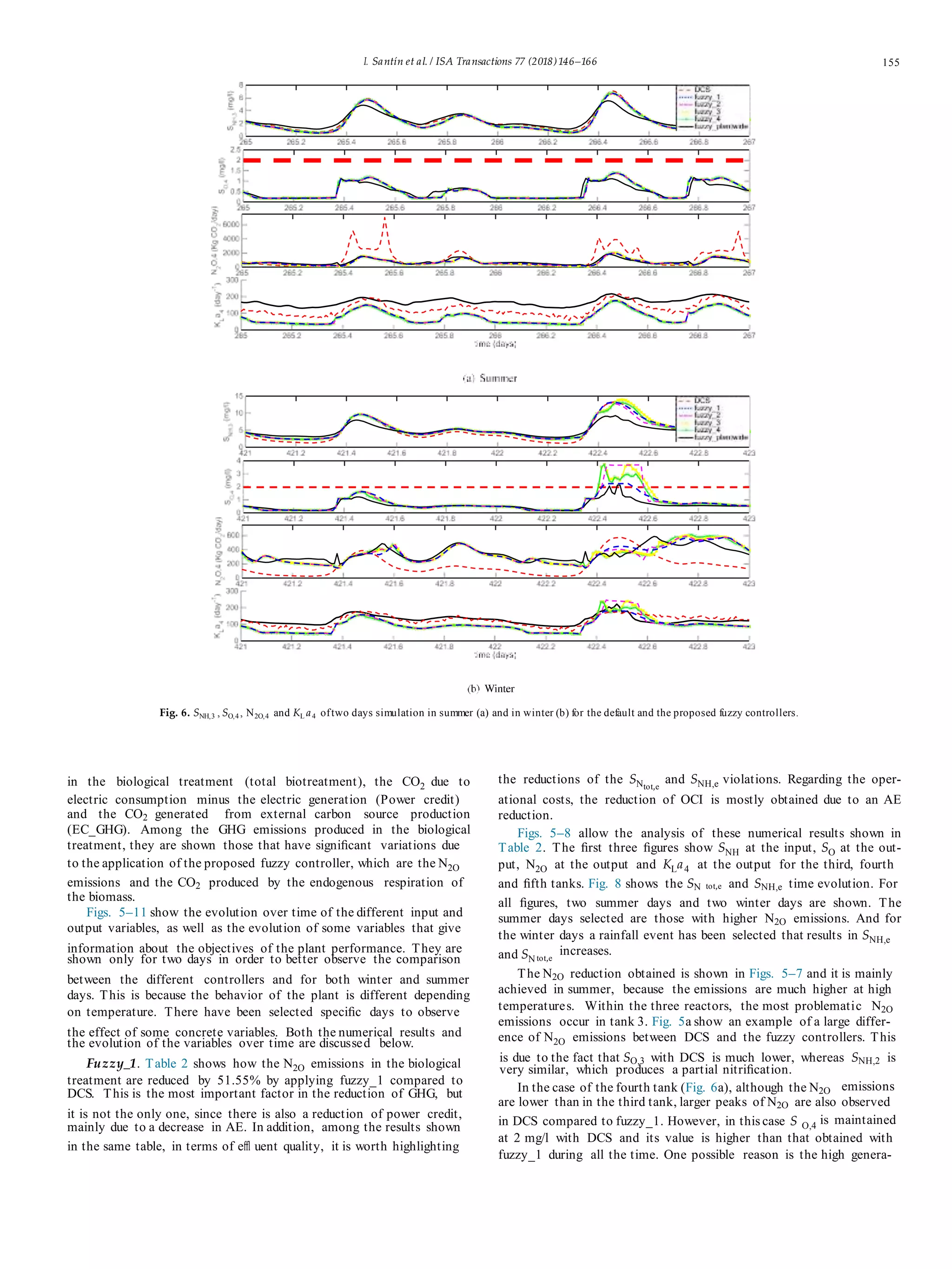
Fuzzy_1. The main objective of fuzzy_1 is to reduce N2O emis-
sions, which are an important factor of GHG emissions. Higher N2O
emissions are generated during nitrification. As shown in several
articles such as Kimochi et al. [3], Kampschreur et al. [4], Foley et
al. [5], Law et al. [6], Flores-Alsina et al. [7,8], Aboobakar et al. [9] or
Wang et al. [10], N2O emissions during nitrification are the result of
partial nitrification. It happens when the SNH oxidation is not com-
pletely converted to SNO3
. Therefore, N2O emissions are related to SO
in the aerobic reactors (Boiocchi et al. [29]).
Therefore, the first application of the fuzzy controller is created
with the intention to avoid partial nitrification. Fuzzy_1 manipulates
the SO set-points of the aerobic reactors based on the SNH input of
each reactor. SO set-points are constrained from 0 to 5 mg/l. The SO
values are finally obtained by the PI controllers, whose set-points
are given by the fuzzy controller. Then, knowing the SNH input of a
reactor and based on the experience of the plant, the required SO is
added by the fuzzy controller for complete nitrification. In addition,
not only the values of SNH, but also their slopes are taken into account
by their derivatives with respect to time. This allows the controller to
be able to act in advance. In the case of fuzzy_1, when SO is low and
SNH begins to increase, the increase of SO has to be fast. Otherwise,
a very large increase of N2O can be produced. For this reason, the
derivative of SNH with respect to time (dSNH/dt) is taken into account,
mainly when the values of SNH are low in order to detect their immi-
nent increase (Fig. 4a, c and e). Finally, the resulting SO values are also
influenced by temperature, because N2O emissions are much higher
at high temperatures (Fig. 4b, d and f). It is important to note the dif-
ference between fuzzy_1 and the cascade SNH control widely used in
the literature (Vrecko et al. [36], Stare et al. [37], Flores-Alsina et al.
[7], Barbu et al. [27], etc.), because although this can achieve better
effl uent quality results, N2O emissions are not considered and par-
tial nitrification can occur, as high GHG emission values are shown
in Barbu et al. [27] by SNH,5 cascade control.
Although the main objective of fuzzy_1 is the reduction of the N2O
emissions, the levels of SNH and SNO3
are also taken into considera-
tion to some extent, since SO is regulated based on the SNH values.
In fuzzy_1 the outputs SO,3, SO,4 and SO,5 have five member-
ship functions, since “very_high” is added in fuzzy_2. Regarding the
1
FIS: Fuzzy Inference System.](https://image.slidesharecdn.com/fuzzy-logic-for-plant-wide-control-of-biological-wastewater-tr2018isa-tran-191011175840/75/Fuzzy-logic-for-plant-wide-control-of-biological-wastewater-treatment-process-including-greenhouse-gas-emissions-6-2048.jpg)
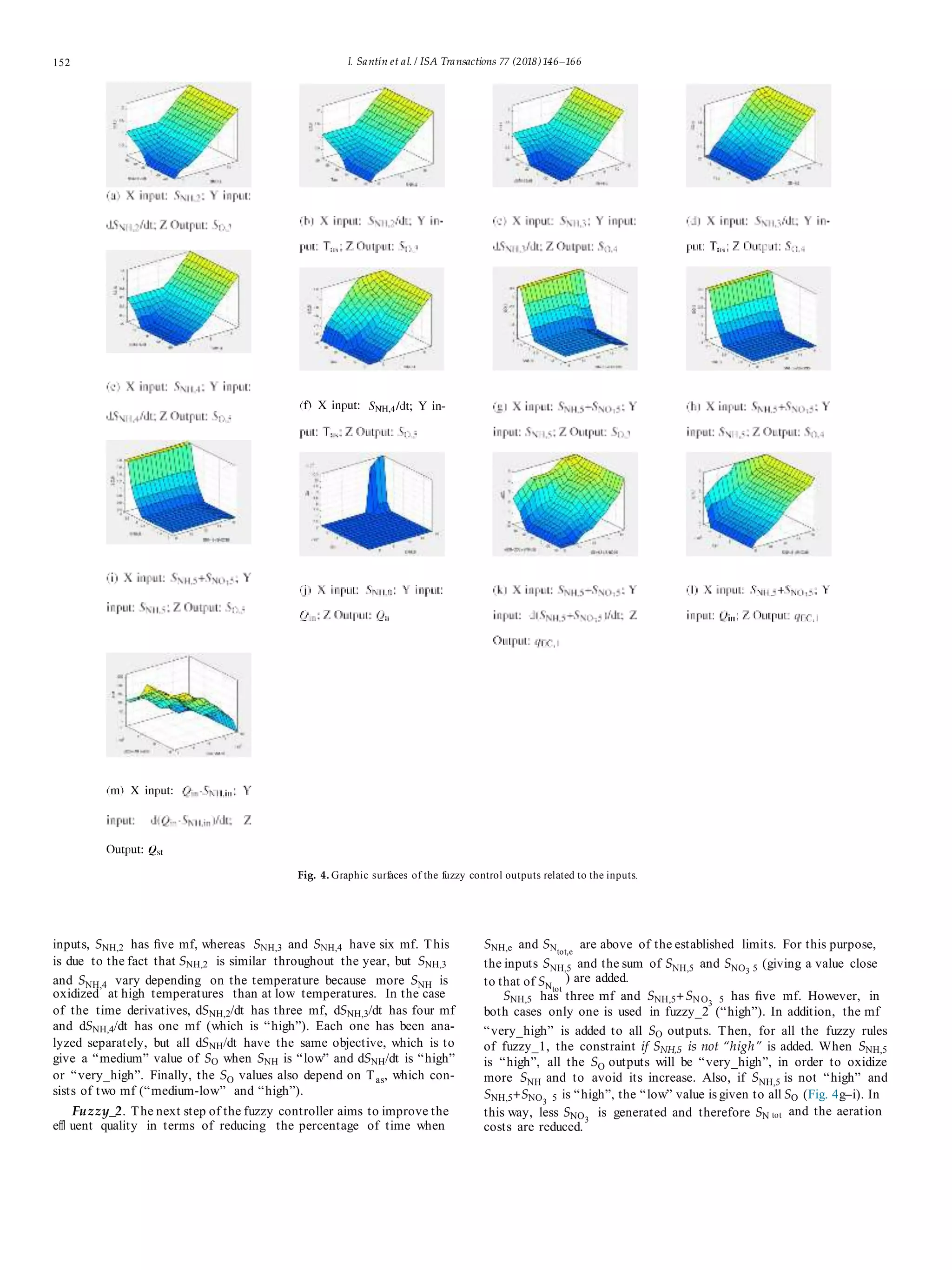
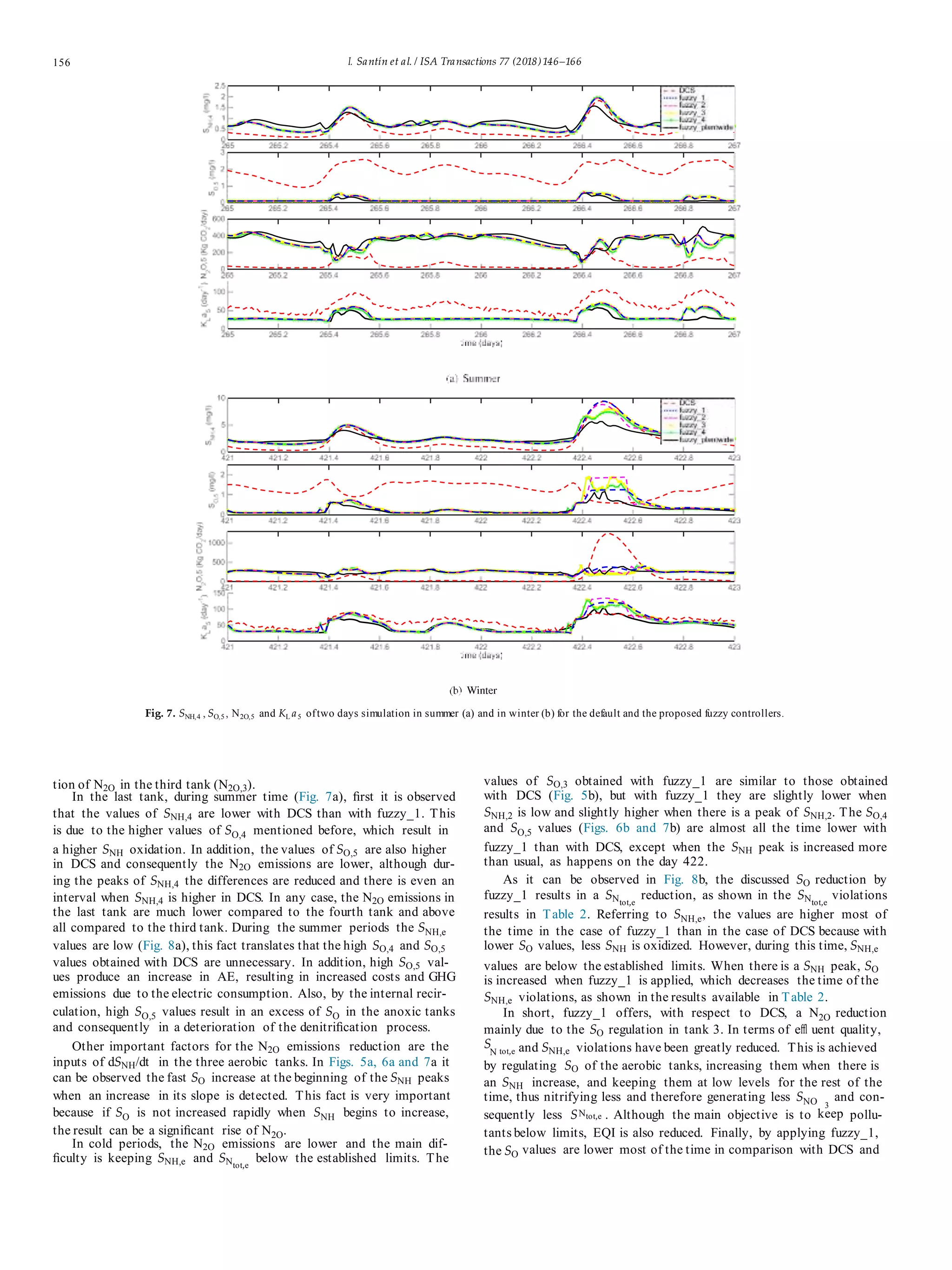
![I. Santín et al. / ISA Transactions 77 (2018)146–166
The input SNH,5+SNO3 5 is not added as a constraint in the fuzzy
rules of fuzzy_1, because that could imply an increase of N2O by
reducing SO.
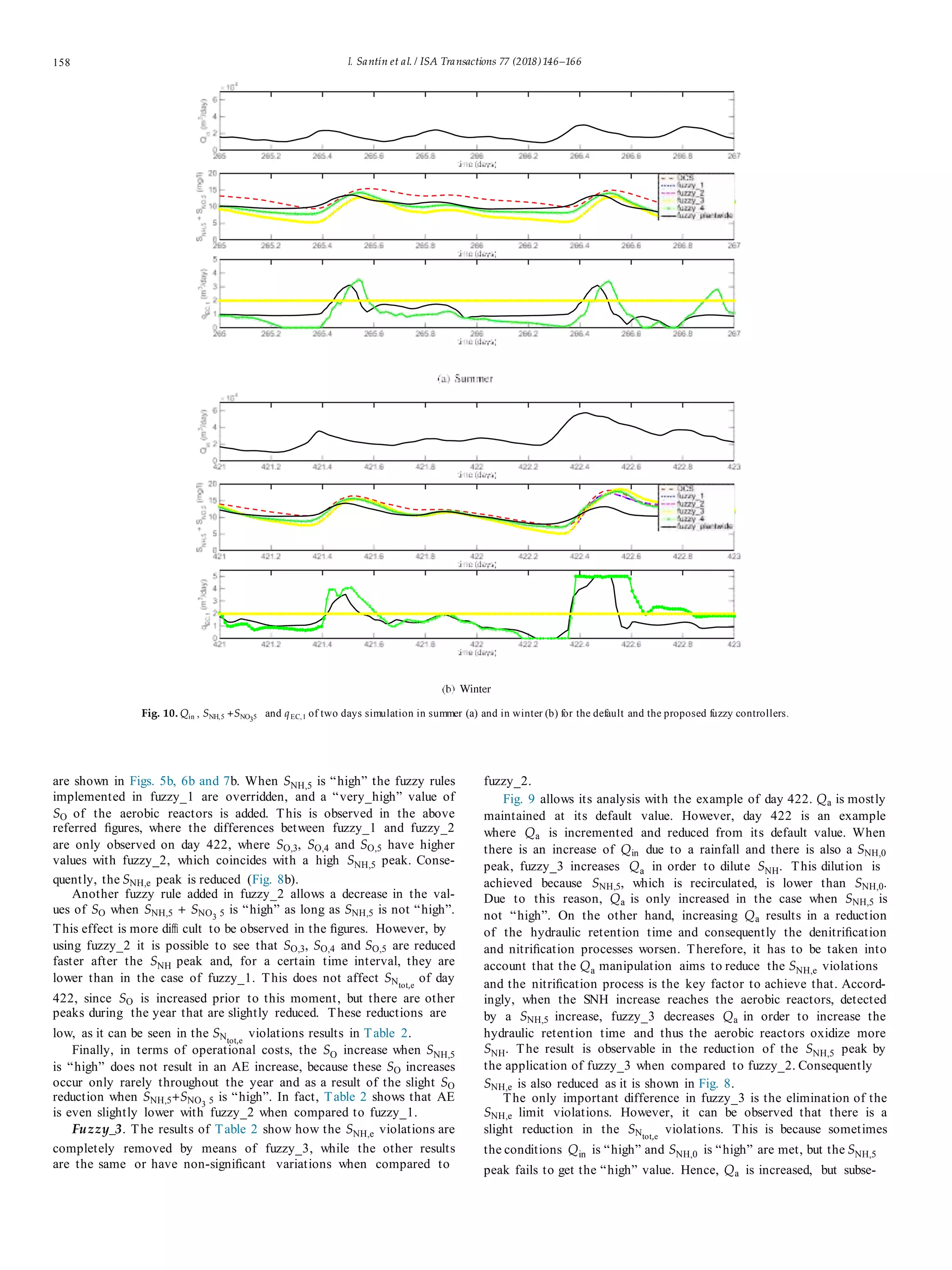
Fuzzy_3. In the following fuzzy controller application, Qa is added
as output, while Qin and SNH,0 are added as inputs. The manipulation
of Qa aims to reduce the SNH peaks and it is not only based on Qin and
SNH,0, but also on SNH,5. Qa is constrained from 0 to 309,720 m3
/d
and, in addition, its variations are also constrained to 26,000 m3
/d
between two samples (15 min) in order not to have abrupt changes.
Qin has one mf (“high”), which is above the usual ranges of dry
weather and, thus, the values of this mf happen when there is rain-
fall event. SNH,0 also has only one mf called “high” and Qa three mf
(“low”, “medium” and “high”). Then, by fuzzy rules, when SNH,5 is
increased close to the limit, Qa is reduced in order to increase the
hydraulic retention time (HRT) and thus improve the nitrification
process. On the other hand, when there is a Qin increase due to a
rainfall and, at that time SNH,0 is “high” while SNH,5 is “low”, Qa is
increased to dilute the SNH concentration (Fig. 4j). When the SNH
peak reaches the aerobic reactors, detected as a result of SNH,5 being
“high”, Qa is reduced.
Fuzzy_4. In fuzzy_4, qEC,1 is added as an output. This is intended to
regulate the addition of qEC,1 instead of keeping it fixed at 2 m3
/d. The
addition of qEC improves the denitrification, significantly reducing
SNO3
values, but on the contrary, it increases the operational costs.
In addition, although a slight decrease of N2O in denitrification can
be produced when external carbon is added, the total GHG emis-
sions are higher due to an increase in the endogenous respiration
of biomass, in the sludge processing and in the chemical and energy
use. Due to these reasons, fuzzy_4 aims to add carbon only in the
cases where a reduction of SNtot,e
is necessary. In this way, the value
of qEC,1 added in fuzzy_4 is based on SNH,5+SN O3 5 and its time deriva-
tive (Fig. 4k). In addition, Qin is also taken into account, since its value
is increased when there is a rainfall, qEC,1 is also increased (Fig. 4l).
The value of qEC,1 is constrained from 0 to 5 m3
/d.
Five mf of the input SNH,5+SNO35 are related to five mf of the
output qEC,1. In the case of d(SNH,5+SNO3 5)/dt, it has three mf and
it is considered both to increase the values of qEC,1 and to reduce
them. So, when the mf of Qin is not active because there is no
rainfall, if d(SNH,5+SNO3 5)/dt is “medium”, the relationship between
SNH,5+SNO3 5 and qEC,1 is as follows: if SNH,5+SNO35 is “low” then qEC,1
is “low”, if SNH,5+SNO3 5 is “medium” then qEC,1 is “medium” and so
on. In the event that d(SNH,5+SNO3 5 )/dt is “high”, qEC,1 is previ-
ously increased to act in advance against SNtot,e
limit violations. If
d(SNH,5+SNO3 5)/dt is “low”, the value of qEC,1 is lower to save carbon
costs. If Qin is “high”, the values of qEC,1 in relation to SNH,5+SNO3 5 and
d(SNH,5+SNO3 5)/dt are also increased.
Fuzzy_plantwide. Finally, the fuzzy controller is fully imple-
mented, which is called fuzzy_plantwide. The fuzzy_plantwide code
is shown in Appendix A and a scheme of its fuzzy rules is in
Appendix B. The last application of the fuzzy controller adds Qst as
a manipulated variable. This is based on the product of Qin and SNH,in
and its derivative with respect to time.
The storage tank is responsible for regulating the amount of
water that is recirculated from the dewatering to the primary settler.
Although the amount of recirculated water is very low in comparison
to the influent, its SNH is very high.
First of all, the default operation of the storage tank has been par-
tially modified. As explained in the previous section, in the default
operation, when the water volume of the tank is below or equal to
the minimum established value, all the flow leads into the tank while
Qst is equal to 0. This has been modified in order to fill the tank if it
is necessary. In such a way that all the flow is led by bypass if Qst
is higher than the input flow. On the other hand, if the given Qst is
lower than the input flow, Qst will be equal to the given value and the
tank will be filled by the difference between the inlet and the out-
153
Table2
Simulationresultsofthedefaultcontrolstrategy,literatureandtheproposedfuzzycontrollersaswellaspercentagesofimprovementwithrespecttothedefaultcontrolstrategy.
EvaluationCriteriaDCSSantínetal.[28]fuzzy_1fuzzy_2fuzzy_3fuzzy_4Fuzzy_plantwide
valuevalue%of
improvement
85.09
value%of
improvement
87.55
value%of
improvement
88.77
value%of
improvement
89.24
value%of
improvement
94.81
value%of
improvement
98,96EffluentqualitySNtot,eviolations
(%ofoperatingtime)
SNH,eviolations
(%ofoperatingtime)
EQI(kgofpollutants/d)
10.61.721.321.191.140.550.11
1.140.05438.570.1289.470.06694.21010001000100
5665.985469.223.475490.453.105489.193.125486.983.165595.431.245567.771.73
OperationalcostsAE(kWh/d)
PE(kWh/d)
EC(kg/d)
OCI
4306.25
261.48
800
9272.78
–
–
–
8635.33
–
–
–
6.94
3788.46
261.48
800
8737.47
12.02
0
0
5.78
3786.08
261.48
800
8735.08
12.08
0
0
5.80
3782.05
263.71
800
8733.22
12.17
−0.85
0
5.82
3701.54
263.74
546.12
7839.63
14.04
−0.86
31.73
15.45
3639.85
263.73
5015.01
7677.35
15.47
−0.86
35.62
17.20
GHGemissionsN2Obiotreatment(kgCO2equiv-
alent/d)
Endogenousrespirationof
biomass(kgCO2/d)
Totalbiotreatment(kgCO2/d)
PowerCredit(kgCO2/d)
EC_GHG(kgCO2/d)
TotalCO2(KgCO2/d)
1596.21197.7922.17773.3751.55782.9250.95786.6650.72801.9249.76858.2846.23
3563.83––3541.010.643540.980.643540.890.643455.733,.033443.693.37
9086.11
−505.85
821.33
17,851.1
–
–
–
17,134.19
–
–
–
4.02
8243.59
−738.91
821.33
16,753.28
9.27
46.07
0
6.15
8253.15
−740.01
821.33
16,761.64
9.18
46.29
0
6.10
8256.82
−740.83
821.33
16,764.53
9.13
46.45
0
6.09
8187.67
−755.23
560.68
16,339.12
9.89
49.30
31.73
8.47
8231.31
−781.23
528.34
16,315.06
9.41
54.44
35.67
8.60](https://image.slidesharecdn.com/fuzzy-logic-for-plant-wide-control-of-biological-wastewater-tr2018isa-tran-191011175840/75/Fuzzy-logic-for-plant-wide-control-of-biological-wastewater-treatment-process-including-greenhouse-gas-emissions-8-2048.jpg)
![154 I. Santín et al. / ISA Transactions 77 (2018)146–166
let flow while the volume does not reach its maximum established
value.
Once the operation of the storage tank has been modified,
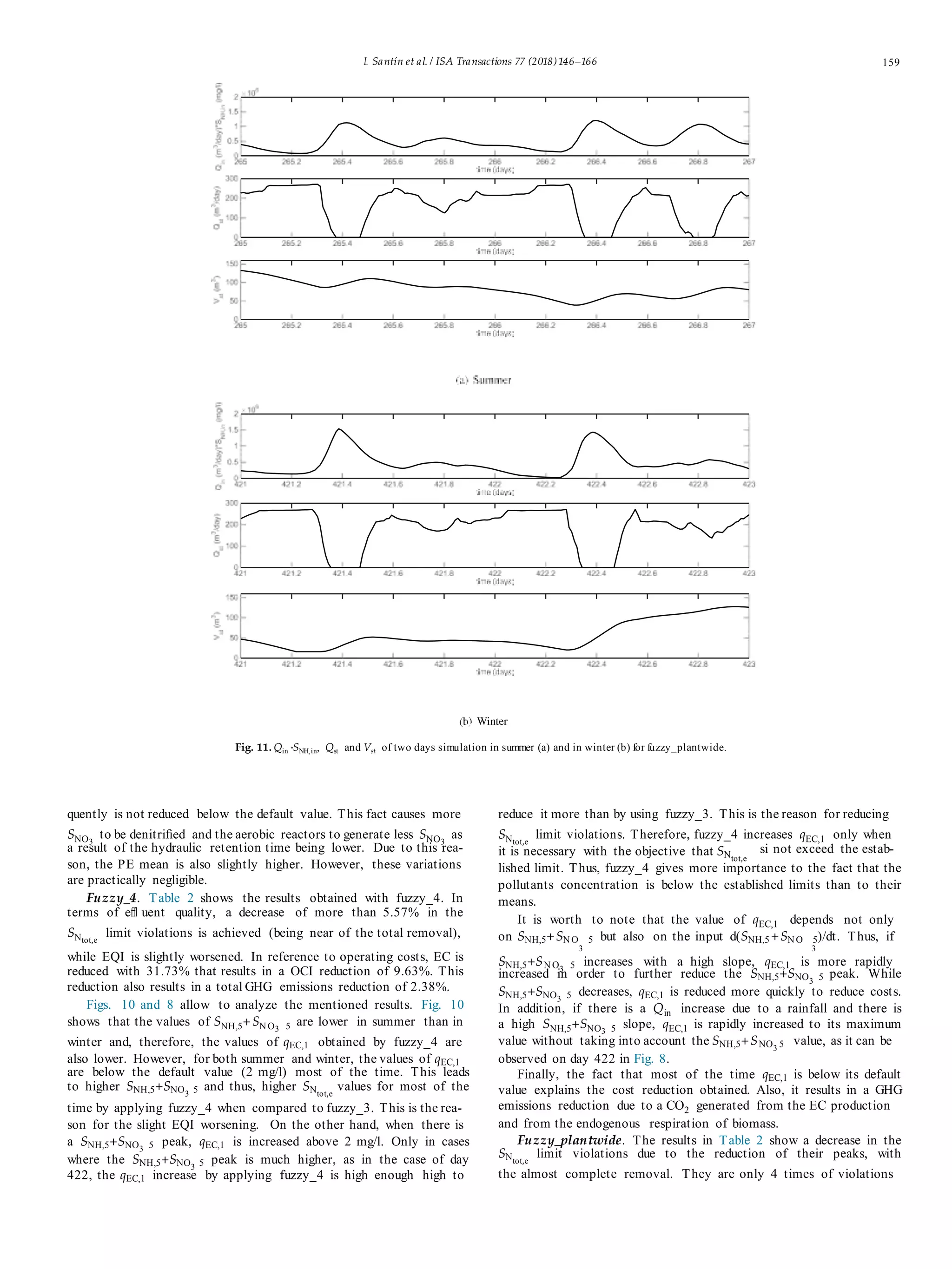
fuzzy_plantwide controller aims to compensate the Qin ·SNH,in peaks
by reducing Qst . Conversely, when the values of Qin ·SNH,in are lower,
Qst is increased to empty the storage tank. Qst is constrained from 0
to 1500 m3
/d.
Both Qin ·SNH,in and Qst have five mf, whereas d(Qin·SNH,in)/dt
has three mf. When d(Qin·SNH,in )/dt is “medium” the relationship
between Qin ·SNH,in and Qst is completely reversed (if Qin ·SNH,in is
“low” then Qst is “high”, if Qin ·SNH,in is “medium-low” then Qst is
“medium-high”, etc). In the case of d(Qin·SNH,in)/dt is “low”, Qst is
higher. Conversely, if d(Qin·SNH,in)/dt is “high”, the values of Qst are
lower (Fig. 4m).
4. Simulation results and discussion
This section presents the simulation results and the discussion
regarding the fuzzy controller. As well as in the previous section, the
results have been analyzed for each one of the fuzzy controllers that
have been implemented incrementally in order to observe the effects
of the different inputs, outputs and fuzzy rules.
Table 2 shows the results obtained with fuzzy_1, fuzzy_2, fuzzy_3,
fuzzy_4 and fuzzy_plantwide, as well as the results of Santín et al.
[28] and DCS. The latter has been used as reference for the percentage
of improvement. The articles Flores-Alsina et al. [7,8] and Boiocchi et
al. [38] also include the GHG emissions assessment, but they have
not been considered for comparison because the first two articles
use the original BSM2G and the last one uses BSM2 for Nitrous oxide
(BSM2N). In the case of Barbu et al. [27] and Santín et al. [28], they
are the only papers that use the same updated BSM2G as the present
article. Although Barbu et al. [27] evaluates GHG emissions, it does
not implement a specific control strategy to reduce them, resulting
in higher GHG emissions than by applying DCS. Therefore, Barbu et
al. [27] has neither been considered for comparison, since the main
objective of the present article is the reduction and consequently, the
first step before considering other criteria.
Effl uent quality has been evaluated through the percentage of
time of SNtot,e
and SNH,e limit violations. Although the main objective
in terms of quality is to keep contaminants below the established
limits, EQI is also shown as a criterion to be compared. COD, TSS and
BOD5 limit violations are not shown because they only occur on cer-
tain days when there is a bypass and this is not modified with the
proposed fuzzy controller.
Within the operational costs, there are shown those that have
significant variations. These are especially AE and EC, but PE is also
shown because Qa is regulated from fuzzy_3.
Regarding the GHG emissions, in addition to the total CO2, the
emissions of the sources that have significant variations with the
proposed fuzzy controller are also shown. These are those produced
Fig. 5. SNH,2 , SO,3 , N2O,3 and KL a3 oftwo days simulation in summer (a) and in winter (b) for the default and the proposed fuzzy controllers.](https://image.slidesharecdn.com/fuzzy-logic-for-plant-wide-control-of-biological-wastewater-tr2018isa-tran-191011175840/75/Fuzzy-logic-for-plant-wide-control-of-biological-wastewater-treatment-process-including-greenhouse-gas-emissions-9-2048.jpg)
![I. Santín et al. / ISA Transactions 77 (2018)146–166 161
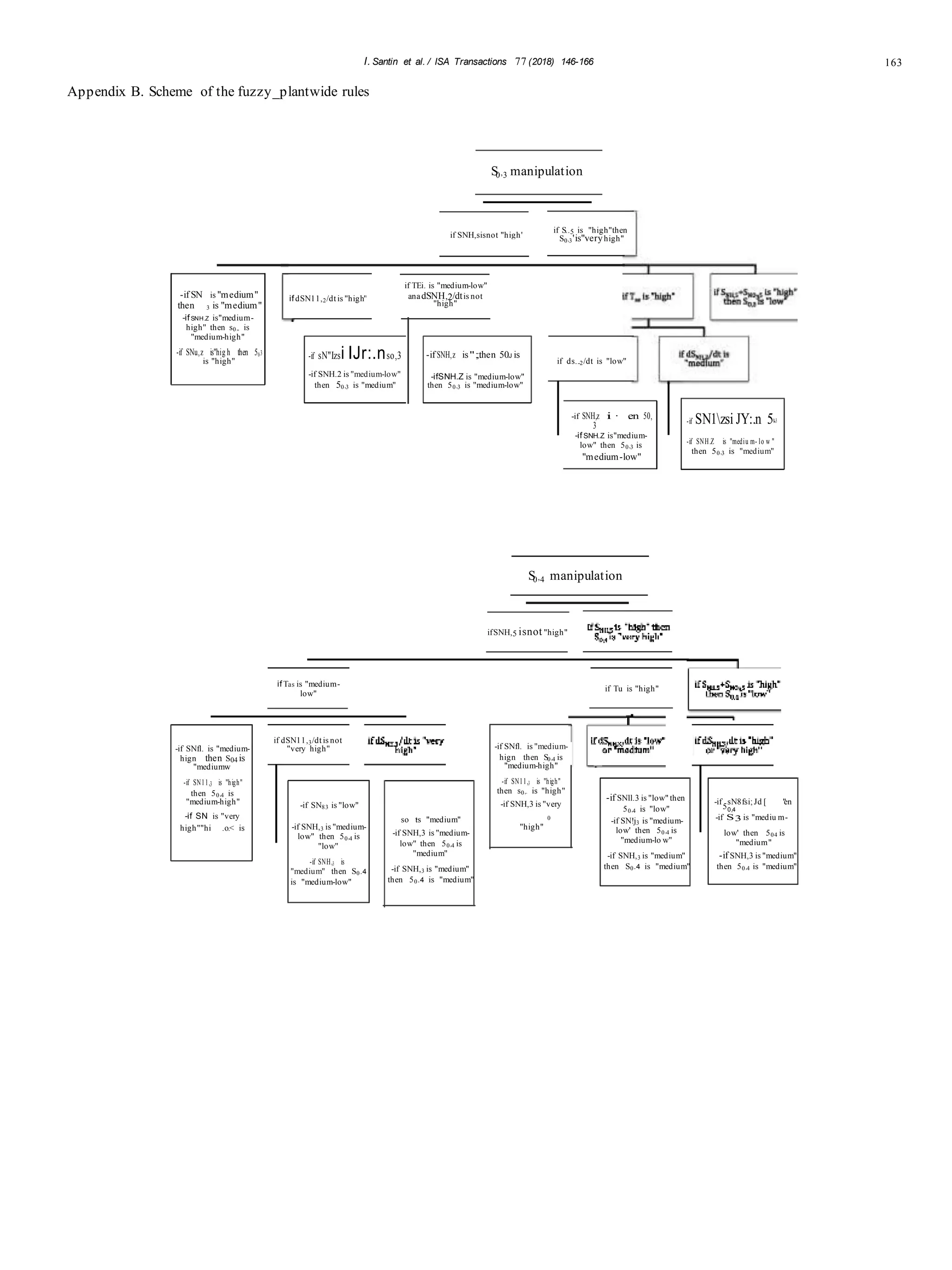
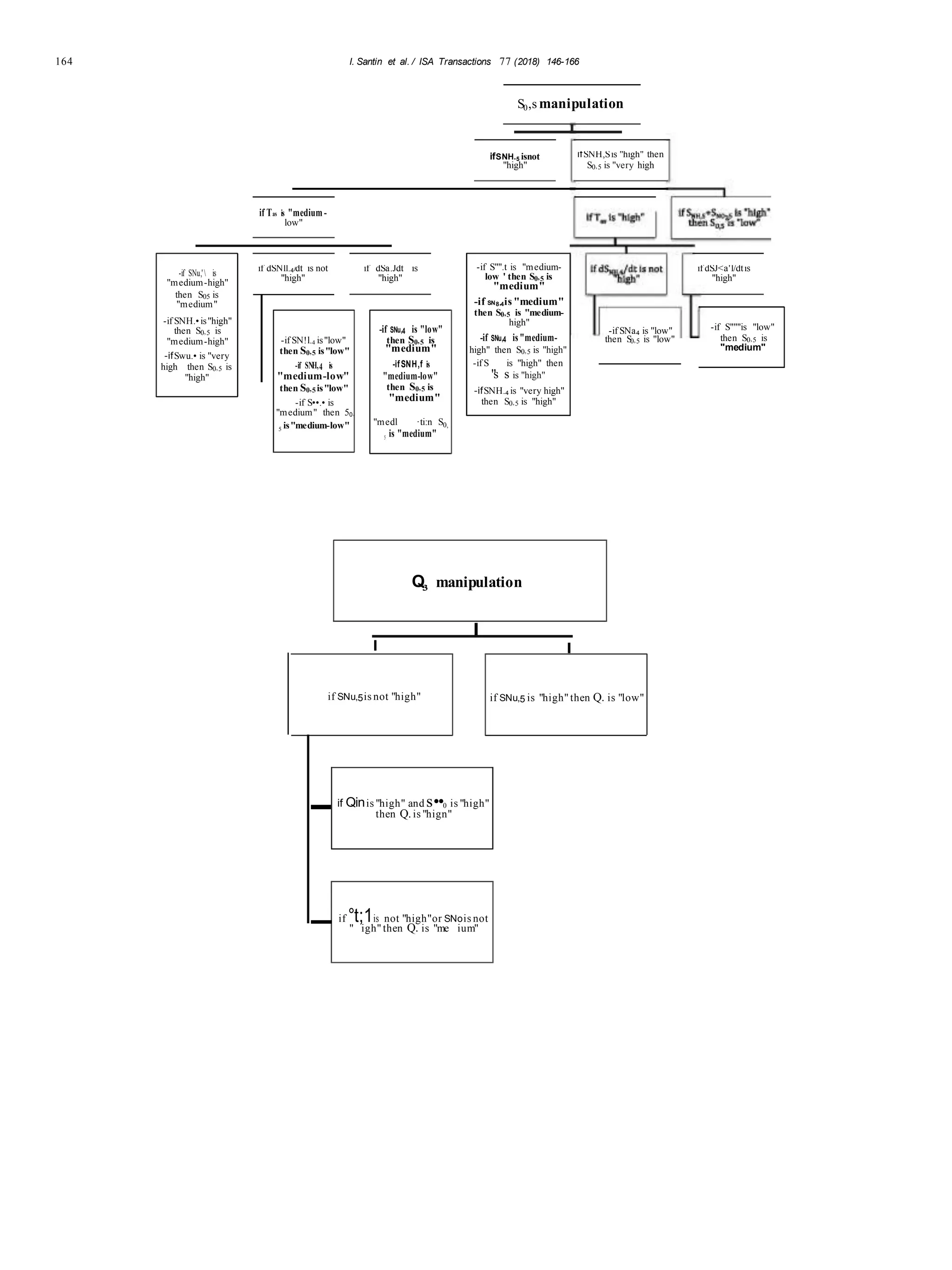
Appendix A. Fuzzy_plantwide code
[System]
Name = ’ Fuzzy_plantwide ’
Type = ’ mamdani ’
Version = 2.0
NumInputs = 14
NumOutputs = 6
NumRules = 80
AndMethod = ’ min ’
OrMethod = ’ max ’
ImpMethod = ’ min ’
AggMethod = ’ max ’
DefuzzMethod = ’ centroid ’
[Input1]
Name = ’ SNH,2 ’
Range = [4 18]
NumMFs = 5
MF1 = ’ low ’ : ’trimf’ , [−1000000 4 7.5]
MF2 = ’ medium−low ’ : ’ trimf’ , [4 7.5 11]
MF3 = ’ medium’ : ’ trimf ’ , [7.5 11 14.5]
MF4 = ’ medium−high ’ : ’ trimf’ , [11 14.5 18]
MF5 = ’ high ’ : ’ trimf’ , [14.5 18 1000000]
[Input2]
Name = ’ SNH,3 ’
Range = [1 12]
NumMFs = 6
MF1 = ’ low ’ : ’ trimf’ , [−1000000 2 3.2]
MF2 = ’ medium−low ’ : ’ trimf’ , [2 3.2 5.4]
MF3 = ’ medium’ : ’ trimf’ , [3.2 5.4 7.6]
MF4 = ’ medium−high ’: ’ trimf’ , [5.4 7.6 9.8]
MF5 = ’ high ’ : ’ trimf’ , [7.6 9.8 12]
MF6 = ’ very_high ’ : ’ trimf’ , [9.8 12 1000000]
[Input3]
Name = ’ SNH,4 ’
Range = [1 7]
NumMFs = 6
MF1 = ’ low ’ : ’ trimf’ , [−1000000 1 2.2]
MF2 = ’ medium−low ’ : ’ trimf’ , [1 2.2 3.4]
MF3 = ’ medium’ : ’ trimf’ , [2.2 3.4 4.6]
MF4 = ’ medium−high ’: ’ trimf’ , [3.4 4.6 5.8]
MF5 = ’ high ’ : ’ trimf’ , [4.6 5.8 7]
MF6 = ’ very_high ’ : ’ trimf’ , [5.8 7 1000000]
[Input4]
Name = ’ dSNH,2/dt ’
Range = [−50 75]
NumMFs = 3
MF1 = ’ low ’ : ’ trimf’ , [−1000000 −50 0]
MF2 = ’ medium’ : ’ trimf ’ , [−37.5 12.5 62.5]
MF3 = ’ high ’ : ’ trimf’ , [25 75 1000000]
[Input5]
Name = ’ dSNH, 3 / dt ’
Range = [−40 60]
NumMFs = 4
MF1 = ’ low ’ : ’ trimf’ , [−1000000 −40–6.667]
MF2 = ’ medium’ : ’ trimf ’ , [−40 −6.667 26.67]
MF3 = ’ high ’ : ’ trimf’ , [20 40 60]
MF4 = ’ very_high ’ : ’ trimf’ , [26.67 60 1000000]
[Input6]
Name = ’ dSNH, 4 / dt ’
Range = [−20 20]
NumMFs = 1
MF1 = ’ high ’ : ’ trimf’ , [10 20 1000000]
(continued on nextpage)
[System]
[Input7] Name
= ’ Tas ’
Range = [10 20]
NumMFs = 2
MF1 = ’ medium− low ’ : ’ trimf ’ , [−1000000 15 20]
MF2 = ’ mf3 ’ : ’ trimf’ , [15 20 1000000]
[Input8]
Name = ’ SNH, 5 ’
Range = [1 4]
NumMFs = 3
MF1 = ’ low ’ : ’ trimf’ , [−1000000 1 2.2]
MF2 = ’ medium’ : ’ trimf’ , [1.3 2.25 3.2]
MF3 = ’ high ’ : ’ trimf’ , [3 3.75 1000000]
[Input9]
Name = ’ SNH, 5 + SNO35 ’
Range = [8 17]
NumMFs = 5
MF1 = ’ low ’ : ’ trimf’ , [−1000000 8 10.26]
MF2 = ’ medium− low ’ : ’ trimf’ , [8 10.26 12.5]
MF3 = ’ medium’ : ’ trimf’ , [10.26 12.5 14.76]
MF4 = ’ medium−high ’ : ’ trimf’ , [12.5 14.76 17]
MF5 = ’ high ’ : ’ trimf’ , [14.76 17 1000000]
[Input10] Name
= ’SNH,0’
Range = [5 14]
NumMFs = 1
MF1 = ’ high ’ : ’ trimf’ , [12 14 1000000]
[Input11]
Name = ’Qin’
Range = [2000 50000]
NumMFs = 1
MF1 = ’ high ’ : ’ trimf’ , [45000 50000 1e+15]
[Input12]
Name = ’ d(SNO35 + SNH,5)/dt ’
Range = [−40 80]
NumMFs = 3
MF1 = ’ low ’ : ’ trimf’ , [−1000000 −40 8]
MF2 = ’ medium’ : ’ trimf’ , [−28 20 68]
MF3 = ’ high ’ : ’ trimf’ , [52.31 80 1000000]
[Input13]
Name = ’ QinSNHin ’ Range
= [200000 1000000]
NumMFs = 5
MF1 = ’ low ’ : ’ trimf’ ,[−1e+16 200000 400000]
MF2 = ’ medium − low ’ : ’ trimf’ , [200000 400000 600000]
MF3 = ’ medium ’ : ’ trimf ’ , [400000 600000 800000]
MF4 = ’ medium−high ’ : ’ trimf’ , [600000 800000 1000000]
MF5 = ’ high ’ : ’ trimf’ , [800000 1000000 1e+16]
[Input14]
Name = ’ d(QinNHin) / dt ’
Range = [−5000000 10000000]
NumMFs = 3
MF1 = ’ low ’ : ’ trimf ’ ,[−1e+17 −5000000 1000000]
MF2 = ’ medium’ : ’ trimf ’ , [−3500000 2500000 8500000]
MF3 = ’ high ’ : ’ trimf ’ , [4000000 10000000 1e+17]
[Output1] Name
= ’ SO, 3 ’
Range = [0 4]
NumMFs = 6
MF1 = ’ low ’ : ’ trimf’ ,[−1000000 0 0.5625]
MF2 = ’ medium− low ’ : ’ trimf’ , [0 0.5625 1.125]
MF3 = ’ medium’ : ’ trimf ’ , [0.5625 1.125 1.688]
MF4 = ’ medium−high ’ : ’ trimf’ , [1.125 1.688 2.25]
MF5 = ’ high ’ : ’ trimf’ , [1.688 2.25 2.813]
MF6 = ’ very_high ’ : ’ trimf’ , [3 3.75 1000000]
(continued on nextpage)](https://image.slidesharecdn.com/fuzzy-logic-for-plant-wide-control-of-biological-wastewater-tr2018isa-tran-191011175840/75/Fuzzy-logic-for-plant-wide-control-of-biological-wastewater-treatment-process-including-greenhouse-gas-emissions-16-2048.jpg)
![162 I. Santín et al. / ISA Transactions 77 (2018)146–166
[System]
[Output2] Name
= ’ SO, 4 ’
Range = [0 4]
NumMFs = 6
MF1 = ’ low ’ : ’ trimf’ , [−1000000 0 0.5625]
MF2 = ’ medium − low ’ : ’ trimf’ , [0 0.5625 1.125]
MF3 = ’ medium’ : ’ trimf ’ , [0.5625 1.125 1.688]
MF4 = ’ medium−high ’ : ’ trimf’ , [1.125 1.688 2.25]
MF5 = ’ high ’ : ’ trimf’ , [1.688 2.25 2.813]
MF6 = ’ very_high ’ : ’ trimf’ , [3 3.75 1000000]
[Output3] Name
= ’ SO, 5 ’
Range = [0 2]
NumMFs = 6
MF1 = ’ low ’ : ’ trimf’ , [−1000000 0 0.3125]
MF2 = ’ medium − low ’ : ’ trimf’ , [0 0.3125 0.625]
MF3 = ’ medium’ : ’ trimf ’ , [0.3125 0.625 0.9375]
MF4 = ’ medium−high ’ : ’ trimf’ , [0.625 0.9375 1.25]
MF5 = ’ high ’ : ’ trimf’ , [0.9375 1.25 1.563]
MF6 = ’ very_high ’ : ’ trimf’ , [1.6 1.85 1000000]
[Output4]
Name = ’ Qa’
Range = [1000 124000]
NumMFs = 3
MF1 = ’ low ’ : ’ trimf’ , [−1e+15 1000 50200]
MF2 = ’ medium ’ : ’ trimf ’ , [13300 62500 111700]
MF3 = ’ high ’ : ’ trimf’ , [74800 124000 1e+15]
[Output5]
Name = ’ qEC, 1 ’
Range = [−0.5 5.5]
NumMFs = 5
MF1 = ’ low ’ : ’ trimf’ , [−1000000 −0.5 1]
MF2 = ’ medium− low ’ : ’ trimf’ , [−0.5 1 2.5]
MF3 = ’ medium’ : ’ trimf’ , [1 2.5 4]
MF4 = ’ medium−high ’ : ’ trimf’ , [2.5 4 5.5]
MF5 = ’ high ’ : ’ trimf’ , [4 5.5 1000000]
[Output6]
Name = ’ Qst ’
Range = [−50 300]
NumMFs = 5
MF1 = ’ low ’ : ’ trimf’ , [−1000000 −50 37.5]
MF2 = ’ medium− low ’ : ’ trimf’ , [−50 37.5125]
MF3 = ’ medium ’ : ’ trimf’ , [37.5 125 212.5]
MF4 = ’ medium−high ’ : ’ trimf’ , [125 212.5300]
MF5 = ’ high ’ : ’ trimf’ , [212.5300 1000000]
[Rules]
1 0 0 −3 0 0 1 −3 0 0 0 0 0 0 , 1 0 0 0 0 0 (1) : 1
2 0 0 −3 0 0 1 −3 0 0 0 0 0 0 , 2 0 0 0 0 0 (1) : 1
3 0 0 0 0 0 0 −3 0 0 0 0 0 0 , 3 0 0 0 0 0 (1) : 1
4 0 0 0 0 0 0 −3 0 0 0 0 0 0 , 4 0 0 0 0 0 (1) : 1
5 0 0 0 0 0 0 −3 0 0 0 0 0 0 , 5 0 0 0 0 0 (1) : 1
1 0 0 1 0 0 2 −3 0 0 0 0 0 0 , 1 0 0 0 0 0 (1) : 1
2 0 0 1 0 0 2 −3 0 0 0 0 0 0 , 2 0 0 0 0 0 (1) : 1
1 0 0 2 0 0 2 −3 0 0 0 0 0 0 , 3 0 0 0 0 0 (1) : 1
2 0 0 2 0 0 2 −3 0 0 0 0 0 0 , 3 0 0 0 0 0 (1) : 1
1 0 0 3 0 0 0 −3 0 0 0 0 0 0 , 3 0 0 0 0 0 (1) : 1
2 0 0 3 0 0 0 −3 0 0 0 0 0 0 , 3 0 0 0 0 0 (1) : 1
0 4 0 0 0 0 2 −3 0 0 0 0 0 0 , 0 4 0 0 0 0 (1) : 1
0 5 0 0 0 0 2 −3 0 0 0 0 0 0 , 0 5 0 0 0 0 (1) : 1
0 1 0 0 1 0 2 −3 0 0 0 0 0 0 , 0 1 0 0 0 0 (1) : 1
0 1 0 0 2 0 2 −3 0 0 0 0 0 0 , 0 1 0 0 0 0 (1) : 1
0 2 0 0 1 0 2 −3 0 0 0 0 0 0 , 0 2 0 0 0 0 (1) : 1
(continued on nextpage)
[System]
0 2 0 0 2 0 2 −3 0 0 0 0 0 0 , 0 2 0 0 0 0 (1) : 1
0 3 0 0 0 0 2 −3 0 0 0 0 0 0 , 0 3 0 0 0 0 (1) : 1
0 1 0 0 3 0 2 −3 0 0 0 0 0 0 , 0 3 0 0 0 0 (1) : 1
0 1 0 0 4 0 2 −3 0 0 0 0 0 0 , 0 3 0 0 0 0 (1) : 1
0 2 0 0 3 0 2 −3 0 0 0 0 0 0 , 0 3 0 0 0 0 (1) : 1
0 2 0 0 4 0 2 −3 0 0 0 0 0 0 , 0 3 0 0 0 0 (1) : 1
0 6 0 0 0 0 0 −3 0 0 0 0 0 0 , 0 5 0 0 0 0 (1) : 1
0 1 0 0 −4 0 1 −3 0 0 0 0 0 0 , 0 1 0 0 0 0 (1) : 1
0 2 0 0 −4 0 1 −3 0 0 0 0 0 0 , 0 1 0 0 0 0 (1) : 1
0 3 0 0 −4 0 1 −3 0 0 0 0 0 0 , 0 2 0 0 0 0 (1) : 1
0 4 0 0 0 0 1 −3 0 0 0 0 0 0 , 0 3 0 0 0 0 (1) : 1
0 5 0 0 0 0 1 −3 0 0 0 0 0 0 , 0 4 0 0 0 0 (1) : 1
0 1 0 0 4 0 1 −3 0 0 0 0 0 0 , 0 3 0 0 0 0 (1) : 1
0 2 0 0 4 0 1 −3 0 0 0 0 0 0 , 0 3 0 0 0 0 (1) : 1
0 3 0 0 4 0 1 −3 0 0 0 0 0 0 , 0 3 0 0 0 0 (1) : 1
0 0 0 0 0 0 0 3 0 0 0 0 0 0 , 6 6 6 0 0 0 (1) : 1
0 0 0 0 0 0 0 −3 5 0 0 0 0 0 , 1 1 1 0 0 0 (1) : 1
0 0 1 0 0 −1 0 −3 0 0 0 0 0 0 , 0 0 1 0 0 0 (1) : 1
0 0 2 0 0 0 2 −3 0 0 0 0 0 0 , 0 0 3 0 0 0 (1) : 1
0 0 3 0 0 0 2 −3 0 0 0 0 0 0 , 0 0 4 0 0 0 (1) : 1
0 0 4 0 0 0 2 −3 0 0 0 0 0 0 , 0 0 5 0 0 0 (1) : 1
0 0 5 0 0 0 2 −3 0 0 0 0 0 0 , 0 0 5 0 0 0 (1) : 1
0 0 6 0 0 0 0 −3 0 0 0 0 0 0 , 0 0 5 0 0 0 (1) : 1
0 0 2 0 0 −1 1 −3 0 0 0 0 0 0 , 0 0 1 0 0 0 (1) : 1
0 0 3 0 0 −1 1 −3 0 0 0 0 0 0 , 0 0 2 0 0 0 (1) : 1
0 0 4 0 0 0 1 −3 0 0 0 0 0 0 , 0 0 3 0 0 0 (1) : 1
0 0 5 0 0 0 1 −3 0 0 0 0 0 0 , 0 0 4 0 0 0 (1) : 1
0 0 1 0 0 1 0 −3 0 0 0 0 0 0 , 0 0 3 0 0 0 (1) : 1
0 0 2 0 0 1 1 −3 0 0 0 0 0 0 , 0 0 3 0 0 0 (1) : 1
0 0 3 0 0 1 1 −3 0 0 0 0 0 0 , 0 0 3 0 0 0 (1) : 1
0 0 0 0 0 0 0 1 0 1 1 0 0 0 , 0 0 0 3 0 0 (1) : 1
0 0 0 0 0 0 0 −3 0 0 −1 0 0 0 , 0 0 0 2 0 0 (1) : 1
0 0 0 0 0 0 0 3 0 0 0 0 0 0 , 0 0 0 1 0 0 (1) : 1
0 0 0 0 0 0 0 2 0 1 1 0 0 0 , 0 0 0 3 0 0 (1) : 1
0 0 0 0 0 0 0 0 1 0 −1 −3 0 0 , 0 0 0 0 1 0 (1) : 1
0 0 0 0 0 0 0 0 2 0 −1 2 0 0 , 0 0 0 0 2 0 (1) : 1
0 0 0 0 0 0 0 0 3 0 −1 2 0 0 , 0 0 0 0 3 0 (1) : 1
0 0 0 0 0 0 0 0 4 0 −1 2 0 0 , 0 0 0 0 4 0 (1) : 1
0 0 0 0 0 0 0 0 5 0 0 0 0 0 , 0 0 0 0 5 0 (1) : 1
0 0 0 0 0 0 0 0 1 0 1 −3 0 0 , 0 0 0 0 3 0 (1) : 1
0 0 0 0 0 0 0 0 2 0 1 −3 0 0 , 0 0 0 0 4 0 (1) : 1
0 0 0 0 0 0 0 0 3 0 1 −3 0 0 , 0 0 0 0 5 0 (1) : 1
0 0 0 0 0 0 0 0 4 0 1 −3 0 0 , 0 0 0 0 5 0 (1) : 1
0 0 0 0 0 0 0 0 1 0 −1 3 0 0 , 0 0 0 0 3 0 (1) : 1
0 0 0 0 0 0 0 0 2 0 −1 3 0 0 , 0 0 0 0 4 0 (1) : 1
0 0 0 0 0 0 0 0 3 0 −1 3 0 0 , 0 0 0 0 4 0 (1) : 1
0 0 0 0 0 0 0 0 4 0 −1 3 0 0 , 0 0 0 0 5 0 (1) : 1
0 0 0 0 0 0 0 0 0 0 1 3 0 0 , 0 0 0 0 5 0 (1) : 1
0 0 0 0 0 0 0 0 2 0 −1 1 0 0 , 0 0 0 0 1 0 (1) : 1
0 0 0 0 0 0 0 0 3 0 −1 1 0 0 , 0 0 0 0 2 0 (1) : 1
0 0 0 0 0 0 0 0 4 0 −1 1 0 0 , 0 0 0 0 3 0 (1) : 1
0 0 0 0 0 0 0 0 0 0 0 0 1 2 , 0 0 0 0 0 5 (1 ): 1
0 0 0 0 0 0 0 0 0 0 0 0 2 2 , 0 0 0 0 0 4 (1 ): 1
0 0 0 0 0 0 0 0 0 0 0 0 3 2 , 0 0 0 0 0 3 (1 ): 1
0 0 0 0 0 0 0 0 0 0 0 0 4 2 , 0 0 0 0 0 2 (1 ): 1
0 0 0 0 0 0 0 0 0 0 0 0 5 0 , 0 0 0 0 0 1 (1 ): 1
0 0 0 0 0 0 0 0 0 0 0 0 1 3 , 0 0 0 0 0 3 (1 ): 1
0 0 0 0 0 0 0 0 0 0 0 0 2 3 , 0 0 0 0 0 3 (1 ): 1
0 0 0 0 0 0 0 0 0 0 0 0 3 3 , 0 0 0 0 0 2 (1 ): 1
0 0 0 0 0 0 0 0 0 0 0 0 4 3 , 0 0 0 0 0 1 (1 ): 1
0 0 0 0 0 0 0 0 0 0 0 0 1 1 , 0 0 0 0 0 5 (1 ): 1
0 0 0 0 0 0 0 0 0 0 0 0 2 1 , 0 0 0 0 0 5 (1 ): 1
0 0 0 0 0 0 0 0 0 0 0 0 3 1 , 0 0 0 0 0 4 (1 ): 1
0 0 0 0 0 0 0 0 0 0 0 0 4 1 , 0 0 0 0 0 3 (1 ): 1](https://image.slidesharecdn.com/fuzzy-logic-for-plant-wide-control-of-biological-wastewater-tr2018isa-tran-191011175840/75/Fuzzy-logic-for-plant-wide-control-of-biological-wastewater-treatment-process-including-greenhouse-gas-emissions-17-2048.jpg)
![I. Santín et al. / ISA Transactions 77 (2018)146–166 165
References
[1] Vilanova R, Santín I, Pedret C. Control y operacin de estaciones depuradoras de
aguas residuales: modelado y simulacin. Revista Iberoamericana de Automtica e
Informtica industrial 2017;14:217–33.
[2] Vilanova R, Santín I, Pedret C. Control en estaciones depuradoras de aguas
residuales: estado actual y perspectivas. Revista Iberoamericana de Automtica
e Informtica industrial 2017;14:329–45.
[3] Kimochi Y, Inamori Y, Mizuochi M, Xu K-Q, Matsumura M. Nitrogen removal
and N2 O emission in a full-scale domestic wastewater treatment plant with
intermittent aeration. J Ferment Bioeng 1998;86(2):202–6.
[4] Kampschreur MJ, Temmink H, Kleerebezem R, Jetten MS, van Loosdrecht
MC. Nitrous oxide emission during wastewater treatment. Water Res
2009;43:4093–103.
[5] Foley J, Yuan Z, Keller J, Senante E, Chandran K, Willis J, Shah A, van Loosdrecht
MCM, van Voorthuizen E. N2 O and CH4 emission from wastewater collection and
treatment systems, Scientific and Technical Report No.30. London, UK: Global
Water Research Coalition; 2011.
[6] Law Y, Ni B, Lant P,Yuan Z.Nitrous oxide(N2 O)production by an enriched culture
of ammonia oxidising bacteria depends on its ammonia oxidation rate. Water Res
2012;46:3409–19.
[7] Flores-Alsina X, Corominas L, Snip L, Vanrolleghem PA. Including greenhouse
gas emissions during benchmarking of wastewater treatment plant control
strategies. Water Res 2011;45(16):4700–10.
[8] Flores-Alsina X, Arnell M, Amerlinck Y, Corominas L, Gernaey KV, Guo L,
Lindblom E, Nopens I, Porro J, Shaw A, Snip L, Vanrolleghem PA, Jeppsson U.
Balancing effl uent quality, economic cost and greenhouse gas emissions during
the evaluation of(plant-wide) control/operational strategies in WWTPs.Sci Total
Environ 2014;466–467:616–24.
[9] Aboobakar A, Cartmell E, Stephenson T, Jones M, Vale P, Dotro G. Nitrous oxide
emissions and dissolved oxygen profiling in a full-scale nitrifying activated
sludge treatment plant. Water Res 2013;47(2):524–34.
[10] Wang Y, Lin X, Zhou D, Ye L, Han H, Song C. Nitric oxide and nitrous oxide
emissions from a full-scale activated sludge anaerobic/anoxic/oxic process. Chem
Eng J 2016;289:330–40.](https://image.slidesharecdn.com/fuzzy-logic-for-plant-wide-control-of-biological-wastewater-tr2018isa-tran-191011175840/75/Fuzzy-logic-for-plant-wide-control-of-biological-wastewater-treatment-process-including-greenhouse-gas-emissions-20-2048.jpg)
![166 I. Santín et al. / ISA Transactions 77 (2018)146–166
[11] Monteith HD, Sahely HR, MacLean HL, Bagley DM. A rational procedure for
estimation of greenhouse-gas emissions from municipal wastewater treatment
plants. Water Environ Res 2005;77:390–403.
[12] Guo L, VanrolleghemPA. Calibration and validation ofan activated sludge model
for greenhouse gases no. 1 (ASMG1): prediction of temperature-dependent N2 O
emission dynamics. Bioproc Biosyst Eng 2014;37:151.
[13] Copp JB. The cost simulation benchmark: description and simulator manual
(COST action 624 and action 682). Luxembourg: Offi ce for Offi cial Publications
od the European Union; 2002.
[14] Gernaey K, Jeppsson U, Vanrolleghem P, Copp J. Benchmarking of control
strategies for wastewater treatment plants, scientific and technical report No.23.
London, UK: IWA Publishing; 2014.
[15] Mannina G, Ekama G, Caniani D, Cosenza A, Esposito G,Gori R, Garrido-Baserba
M, Rosso D, Olsson G. Greenhouse gases from wastewater treatment - a review
of modelling tools. Sci Total Environ 2016;551:254–70.
[16] Ni B-J, Yuan Z. Recent advances in mathematical modeling of nitrous oxides
emissions from wastewater treatment processes. Water Res 2015;87:336–46.
[17] BelchiorCAC,Araújo RAM,Landeck JAC.Dissolved oxygen control oftheactivated
sludge wastewater treatment process using stable adaptive fuzzy control.
Comput Chem Eng 2012;37:152–62.
[18] Nasr M, Moustafa M, Seif H, El-Kobrosy G. Application offuzzy logic control for
benchmark simulation model. 1. Sustain Environ Res 2014;24.
[19] Traore A, Grieu S, Puig S, Corominas L, Thiéry F, Polit M, Colprim J. Fuzzy
control of dissolved oxygen in a sequencing batch reactor pilot plant. Chem Eng
J 2005;111:13–9.
[20] Santín I, Pedret C, Vilanova R. Applying variable dissolved oxygen set point in
a two level hierarchical control structure to a wastewater treatment process. J
Process Control 2015;28:40–55.
[21] Meyer U, Pöpel H. Fuzzy-control for improved nitrogen removal and energy
saving in wwt-plants with pre-denitrification. Water Sci Technol 2003;47:
69–76.
[22] Pai T, Wan T, Hsu S, Chang T,Tsai Y,Lin C,Su H,Yu L.Using fuzzy inferencesystem
to improve neural network for predicting hospital wastewater treatment plant
effl uent. Comput Chem Eng 2009;33:1272–8.
[23] Santín I, Pedret C, Vilanova R. Fuzzy control and model predictive control
configurations for effl uent violations removal in wastewater treatment plants.
Ind Eng Chem Res 2015;54(10):2763–75.
[24] Santín I, Pedret C, Vilanova R, Meneses M. Advanced decision control systemfor
effl uent violations removal in wastewater treatment plants. Control Eng Pract
2016;279:207–19.
[25] Kalavrouziotis I, Pedrero F, Skarlatos D. Water and wastewater quality
assessment based on fuzzy modeling for the irrigation of Mandarin. Desalination
Water Treat 2016;57:20159–68.
[26] Hirsch P, Piotrowski R, Duzinkiewicz K, Grochowski M. Supervisory control
system for adaptive phase and work cycle management of sequencing
wastewater treatment plant. Stud Inf Control 2016;25:153–62.
[27] Barbu M, Vilanova R, Meneses M, Santin I. On the evaluation of the global
impact of control strategies applied to wastewater treatment plants. J Clean Prod
2017;149:396–405.
[28] Santín I, Barbu M, Pedret C, Vilanova R. Control strategies for nitrous oxide
emissions reduction on wastewater treatment plants operation. Water Res
2017;125:466–77.
[29] Boiocchi R, Gernaey KV, Sin G. Understanding N2 O formation mechanisms
through sensitivity analyses using a plant-wide benchmark simulation model.
Chem Eng J 2017;317:935–51.
[30] Henze M, Grady C, Gujer W, Marais G, Matsuo T. Activated sludge model 1,
scientific and technical report No.1. London, UK: IAWQ; 1987.
[31] Hiatt W, Grady JC. An updated process model for carbon oxidation, nitrification,
and denitrification. Water Environ Res 2008;80(11):2145–56.
[32] Mampaey KE, Beuckels B, Kampschreur RKMJ, van Loosdrecht MC, Volcke EI.
Modelling nitrous and nitric oxide emissions by autotrophic ammonia-oxidizing
bacteria. Environ Technol 2013;34(12):1555–66.
[33] Nopens I, Benedetti L, Jeppsson U, Pons M-N, Alex J, Copp JB, Gernaey KV,
Rosen C, Steyer J-P, Vanrolleghem PA. Benchmark Simulation Model No 2:
finalisation of plant layout and default control strategy. Water Sci Technol
2010;62(9):1967–74.
[34] KlirG, Yuan B. Fuzzy sets and fuzzy logic,vol.4.New Jersey: PrenticeHall; 1995.
[35] Mamdani E. Application offuzzy algorithms for control ofsimple dynamic plant.
Proc Inst Electr Eng 1976;121(12):1585–8.
[36] Vrecko D, Hvala N, Stare A, Burica O, Strazar M, Levstek M, Cerar P, Podbevsek
S. Improvement of ammonia removal in activated sludge process with feedfor-
ward-feedback aeration controllers.Water Sci Technol 2006;53(4–5):125–32.
[37] Stare A, Vrecko D, Hvala N, Strmcnick S. Comparison of control strategies for
nitrogen removal in an activated sludge process in terms of operating costs: a
simulation study. Water Res 2007;41(9):2004–14.
[38] Boiocchi R, Gernaey KV, Sin G.Control ofwastewater n 2 o emissions by balancing
the microbial communities using a fuzzy-logic approach. IFAC-PapersOnLine
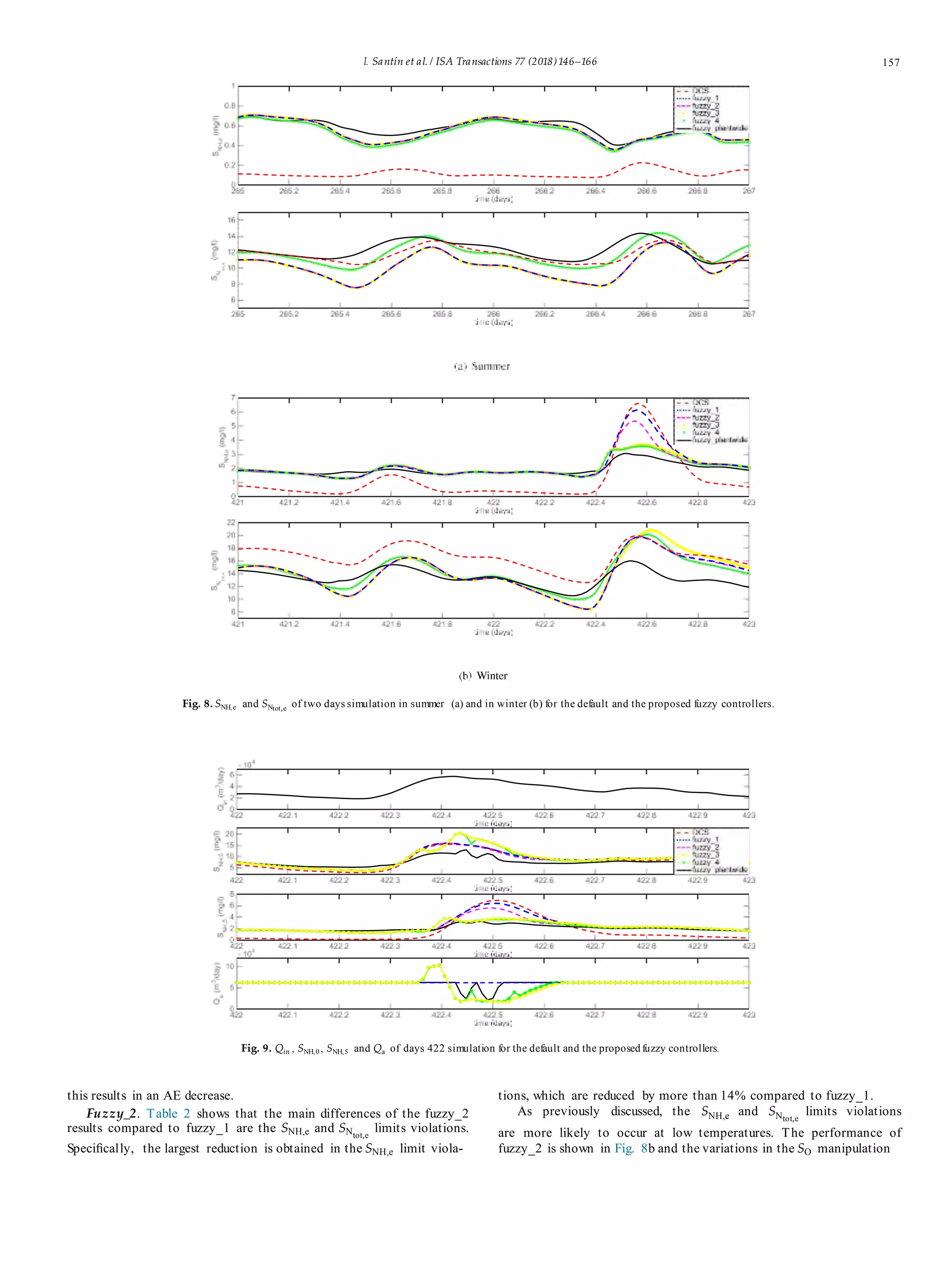
2016;49:1157–62.](https://image.slidesharecdn.com/fuzzy-logic-for-plant-wide-control-of-biological-wastewater-tr2018isa-tran-191011175840/75/Fuzzy-logic-for-plant-wide-control-of-biological-wastewater-treatment-process-including-greenhouse-gas-emissions-21-2048.jpg)

The article presents a fuzzy controller for the plant-wide control of biological wastewater treatment processes, focusing on the reduction of greenhouse gas emissions, particularly nitrous oxide and carbon dioxide. Using a benchmark simulation model, the developed controller integrates 14 inputs and 6 outputs to improve effluent quality and operational costs while addressing greenhouse gas emissions. Results demonstrate that the fuzzy controller effectively reduces emissions while maintaining satisfactory treatment outcomes.