This research article presents a novel adaptive PID controller design utilizing fuzzy models for the control of nonlinear and uncertain processes, specifically applied to industrial settings. The proposed method employs a fuzzy predictor to adjust the PID gains based on real-time input-output data, enhancing tracking performance and robustness to noise while eliminating the need for a first-principal model of the process. Performance tests on a bioreactor demonstrate the method's effectiveness in managing instabilities and parameter variations in nonlinear systems.

1. Research Article
A fuzzy model based adaptive PID controller design for nonlinear
and uncertain processes
Aydogan Savran n
, Gokalp Kahraman 1
Department of Electrical and Electronics Engineering, Ege University, 35100 Bornova, Izmir, Turkey
a r t i c l e i n f o
Article history:
Received 19 September 2012
Received in revised form
16 September 2013
Accepted 26 September 2013
Available online 17 October 2013
This paper was recommended for
publication by Prof. A.B. Rad
Keywords:
Adaptive
PID
Fuzzy
Prediction
Soft limiter
LM
BPTT
Control
a b s t r a c t
We develop a novel adaptive tuning method for classical proportional–integral–derivative (PID)
controller to control nonlinear processes to adjust PID gains, a problem which is very difficult to
overcome in the classical PID controllers. By incorporating classical PID control, which is well-known in
industry, to the control of nonlinear processes, we introduce a method which can readily be used by the
industry. In this method, controller design does not require a first principal model of the process which is
usually very difficult to obtain. Instead, it depends on a fuzzy process model which is constructed from
the measured input–output data of the process. A soft limiter is used to impose industrial limits on the
control input. The performance of the system is successfully tested on the bioreactor, a highly nonlinear
process involving instabilities. Several tests showed the method's success in tracking, robustness to noise,
and adaptation properties. We as well compared our system's performance to those of a plant with
altered parameters with measurement noise, and obtained less ringing and better tracking. To conclude,
we present a novel adaptive control method that is built upon the well-known PID architecture that
successfully controls highly nonlinear industrial processes, even under conditions such as strong
parameter variations, noise, and instabilities.
& 2013 ISA. Published by Elsevier Ltd. All rights reserved.
1. Introduction
PID controllers are well-known and popular in industry due to
their simplicity and robustness, but most of them lack well-tuning
and accuracy, that motivated much work to develop tuning and
adaptation techniques to cope with nonlinear industrial processes
[1–8]. Adaptive tuning becomes necessary for parameter varia-
tions, which fixed parameter controllers cannot sufficiently com-
pensate. Recently, predictive control technique has been widely
appeared in the process control [9–11]. In the predictive control, a
process model is required to predict the future effects of the
control action at the present. First principles-based nonlinear
models are difficult to develop for many industrial cases. Non-
linear process can be alternatively modeled with fuzzy systems.
Fuzzy logic was introduced by Zadeh [12,13] and then used for
many control and modeling applications [14,15]. Takagi–Sugeno
[16] and Mamdani [17] fuzzy models are the two main types of
fuzzy systems. The Takagi–Sugeno fuzzy model (Takagi–Sugeno
modeling methodology) includes fuzzy sets only in the premise
part and a regression model as the consequent [16] while the
Mamdani fuzzy model includes fuzzy sets in both parts. Many
successful applications of the predictive control using fuzzy
models have been reported in the literature [18–21].
Although, the PID tuning and adaptation techniques have exten-
sively developed for linear time-invariant systems [2,3,22–26],
still much effort should be spent for nonlinear as well as time-
variant systems. This has motivated this study. In this paper, a
novel adaptive tuning procedure for classical PID controllers is
developed and efficiently applied for a nonlinear process control
problem. One of the main features of the proposed approach is
that the PID controller architecture is solely classic making it
readily usable in nonlinear industrial processes, avoiding lengthy
and less familiar fuzzy systems. Our classic PID design allows
computing the parameters from the measured input–output data
of the nonlinear process more precisely than other known designs
by virtue of its multi-step forward prediction, on-line predictor
training, adaptive controller tuning, and fast training features. By
this way, a predictive adjustment procedure is performed based on
the predictions of a fuzzy model of the process. Adaptation part
involves a classical PID controller driving a fuzzy predictor. The
fuzzy predictor output is used to adjust the gains by minimizing the
error between the predictions and the reference. Additionally, the
fuzzy predictor is trained on-line to adapt to the variations in plant
parameters, and thus improve the prediction accuracy. The actual
plant is controlled by a PID controller identical to that of the
Contents lists available at ScienceDirect
journal homepage: www.elsevier.com/locate/isatrans
ISA Transactions
0019-0578/$ - see front matter & 2013 ISA. Published by Elsevier Ltd. All rights reserved.
http://dx.doi.org/10.1016/j.isatra.2013.09.020
n
Corresponding author. Tel.: þ90 232 3111664; fax: þ90 232 3886024.
E-mail addresses: aydogan.savran@ege.edu.tr (A. Savran),
gokalp.kahraman@ege.edu.tr (G. Kahraman).
1
Tel.: þ90 232 3111669; fax: þ90 232 3886024.
ISA Transactions 53 (2014) 280–288

2. adaptation part, the gains of which are transferred at each control
cycle. A soft limiter is used to impose industrial limits on the
control input.
In a concurrent work [27], we have used a fuzzy system to
implement the controller that resulted in procedurally lengthy and
computationally heavy algorithms that are unfavorable in industrial
users. In contrast, in this work simple PID gain parameters replace
lengthy fuzzy-system computations. The predictor is constructed
only from the measurement of the input–output data of the actual
process as a fuzzy model, without requiring a first-principal model of
the process which is usually very difficult to obtain.
Section 2 provides background information on the structure of
the fuzzy systems and the PID controller, used in the paper,
whereas Section 3 explains the control system architecture and
the training procedure. Section 4 discusses the results of the
performance tests done on the bioreactor, a highly nonlinear
process involving instabilities. Several tests and comparative study
showed the method's success in tracking, robustness to noise, and
adaptation properties. Section 5 is the conclusion, summarizing
the performance of our method.
2. The background
2.1. The PID controller
Proportional–integral–derivative (PID) controllers, which have
relatively simple structures and robust performances, are the most
common controllers in industry. By taking the time-derivative of
the both sides of the continuous-time PID equation, and discretiz-
ing the resulting equation, one easily gets the PID equation in the
incremental form as below:
uðkÞ ¼ uðkÀ1ÞþKPðeðkÞÀeðkÀ1ÞÞþ
KIT
2
ðeðkÞþeðkÀ1ÞÞ
þ
KD
T
ðeðkÞÀ2eðkÀ1ÞþeðkÀ2ÞÞ ð1Þ
where KP is the proportional gain, KI is the integral gain, and KD is
the derivative gain. T is the sampling period, u is the output of the
PID controller, and k is the discrete time index. The difference
between the reference input (r) and the actual plant output (y) is
the error term, e¼rÀy. Equation can be simplified to
ΔuðkÞ ¼ KPePðkÞþKIeIðkÞþKDeDðkÞ
uðkÞ ¼ uðkÀ1ÞþΔuðkÞ ð2Þ
where
ePðkÞ ¼ eðkÞÀeðkÀ1Þ
eIðkÞ ¼
T
2
ðeðkÞþeðkÀ1ÞÞ
eDðkÞ ¼
1
T
ðeðkÞÀ2eðkÀ1ÞþeðkÀ2ÞÞ ð3Þ
with eðkÞ ¼ 0 for ko0.
In order to provide the control signal in physical limits, a soft
limiter is placed after the controller. The control signal at the
output of the soft limiter becomes
ulðkÞ ¼ hðuðkÞÞ ð4Þ
where hðuÞ ¼ 1=1þeÀu
is a sigmoid type function.
2.2. The fuzzy system
The fuzzy system (FS), f ðx; θÞ, used in this study consists of the
product inference engine, the singleton fuzzifier, the center average
defuzzifier, and the Gaussian membership functions [28,29]:
f ðxðkÞ; θÞ ¼
∑M
j ¼ 1bj∏N
i ¼ 1expðÀ1
2 ðxiðkÞÀcij=sijÞ2
Þ
∑M
j ¼ 1∏N
i ¼ 1expðÀ1
2 ðxiðkÞÀcij=sijÞ2
Þ
ð5Þ
where xi is the ith input of the FS, N is the number of inputs, M is the
number of membership functions assigned to each input, cij and sij
are, respectively, the center and the spread of the jth membership
function corresponding to the ith input. Any output membership
function which has a fixed spread of 1 is characterized only by the
center parameter bj. The input vector x(k) represents all of the inputs
of the FS at time k. The parameter vector θ ¼ ½b; c; rŠ contains all of
the fuzzy-set parameters. The derivatives ð∂f ðxðkÞ; θÞ=∂θÞ for the FS
output with respect to its parameters are computed as
∂f
∂bj
¼
∂f
∂α
∂α
∂bj
¼
1
ϕ
zj
∂f
∂cij
¼
∂f
∂zj
∂zj
∂cij
¼
ðbj Àf Þ
ϕ
zj
ðxi ÀcijÞ
ðsijÞ2
∂f
∂sij
¼
∂f
∂zj
∂zj
∂sij
¼
ðbj Àf Þ
ϕ
zj
ðxi ÀcijÞ2
ðsijÞ3
ð6Þ
where
zj ¼ ∏N
i ¼ 1expðÀ1
2 ðxi Àcij=sijÞ2
Þ
α ¼ ∑M
j ¼ 1bjzj
φ ¼ ∑M
j ¼ 1zj
f ¼
α
φ
ð7Þ
The input–output sensitivities of the FS are computed as
∂f ðxÞ
∂xi
¼ ∑M
j ¼ 1
f ðxÞÀbj
φ
zj
xi Àcij
s2
ij
!
ð8Þ
3. The adaptive PID control system
3.1. Control system architecture
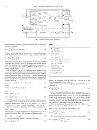
Fig. 1 depicts the adaptive PID control system architecture. The
adaptation part includes the PID controller and the fuzzy predictor.
The PID controller computes the control actions. The predictor is
constructed only from the measurement of the input–output data
of the actual process as a fuzzy model, without requiring a first-
principal model of the process which is usually very difficult to
obtain. The multi-step ahead predictions of the process output are
provided by the fuzzy predictor. The fuzzy predictor output is used
to adjust the gains by minimizing the sum of the squared errors
between the predictions and the reference over the prediction
horizon. The fuzzy predictor is trained on-line to adapt to the
variations in plant parameters, and thus improve the prediction
accuracy. A certain history of the actual plant inputs and outputs is
stored in a first-in first-out stack, providing the online training
data at each training step [30]. The PID controller gains and the
predictor fuzzy system parameters are both adjusted by the
Levenberg–Marquardt (LM) method [31]. The actual plant is
controlled by a PID controller identical to that of the adaptation
phase, the gains of which are transferred at each control cycle.
A sigmoid-type soft limiter is used to impose industrial limits on
the control input.
3.2. Adaptation of the PID controller gains
The fuzzy predictor parameters and the controller gains are
adjusted at each control cycle. The cost function used to adjust
the controller gains is defined as the sum of the squared error
A. Savran, G. Kahraman / ISA Transactions 53 (2014) 280–288 281

3. between the set point and the predictor output over the prediction
horizon H as below:
EH
c ¼
1
2H
∑
H À1
n ¼ 0
ðrðkþnÞÀ ^yðkþnÞÞ2
ð9Þ
where k is the initial edge of the prediction horizon. The Jacobian
with respect to the controller gains θc
¼ ½Kp; KI; KDŠ is computed as
Jc ¼
∂^e
∂θc ¼
∂^e
∂f p
∂f p
∂^ul
∂^ul
∂^u
∂^u
∂θc ð10Þ
One should notice that the delay elements at the outputs of PID
controller and the fuzzy predictor form recurrent systems, and as
such their Jacobians (or equivalently gradients) are computed by
the back-propagation through time (BPTT) method which is based
on the adjoint model.
The Jacobians ðJc ¼ ∂^e=∂θc
Þ are computed in two phases referred
as the forward and the backward. In the forward phase, at every
time step k, the controller and predictor sequentially run and their
outputs are stored from n¼0 to n¼HÀ1, where n counts the
ahead of time steps and H is the prediction horizon. The ahead-of-
time value of control signal, denoted as ^uðnÞ, drives the predictor,
and it is given by
^uðnÞ ¼ ^uðnÀ1ÞþΔ^uðnÞ; for n ¼ 0; 1; :::; HÀ1 ð11Þ
where
Δ^uðnÞ ¼ KP ^ePðnÞþKI ^eIðnÞþKD ^eDðnÞ ð12Þ
^epðnÞ ¼ ^eðnÞÀ ^eðnÀ1Þ
^eIðnÞ ¼
T
2
ð^eðnÞþ ^eðnÀ1ÞÞ
^eDðnÞ ¼
1
T
ð^eðnÞÀ2^eðnÀ1Þþ ^eðnÀ2ÞÞ ð13Þ
The difference between the reference and the predictor output,
^eðnÞ ¼ rðkþnÞÀ ^yðkþnÞ is the ahead-of-time error. The initial con-
ditions of the equations from (11) to (12) are ^uðn ¼ À1Þ ¼ uðkÀ1Þ
^eðn ¼ 0Þ ¼ eðkÀ1Þ, ^eðn ¼ À1Þ ¼ eðkÀ2Þ, and ^eðn ¼ À2Þ ¼ eðkÀ3Þ.
The control action at the output of the limiter is obtained as
^ulðnÞ ¼ hð^uðnÞÞ; ð14Þ
where limiter h is a sigmoid type function. The predictor input vector
contains the control action and the previous predictor output:
^x
p
ðnÞ ¼ ½^yðkþnÀ1Þ; ^ulðnÞŠ ð15Þ
The predicted plant output is the predictor output:
^yðkþnÞ ¼ f pð^x
p
ðnÞ; θp
Þ ð16Þ
where the parameter vector θp
¼ ½b
p
; cp
; rp
Š contains all of the
fuzzy-set parameters of the predictor.
The mean square error through the prediction horizon is
computed as
EH
c ¼
1
2H
∑
H À1
n ¼ 0
^e
2
ðnþ1Þ ð17Þ
Table 1 summarizes the forward phase computations.
At the completion of the forward phase at each k, the backward
phase computations from n ¼ HÀ1 to n ¼ 0 are performed by
means of the adjoint model shown in Fig. 2. In the adjoint model,
the arrow directions of the signal propagation are reversed, the
summing junctions and the branching points are interchanged,
and the advance operators replace the delay operators.
The backward action at the predictor output is obtained as
δpðnÞ ¼ ½À1þvðnþ1ÞŠ; for n ¼ HÀ1; :::; 0: ð18Þ
with vðn ¼ HÞ ¼ 0. The vðnÞ is computed via δpðnÞ:
vðnÞ ¼
∂f pðxp
; θp
Þ
∂xp
1

8. ^x
p
ðnÞ
δpðnÞ ð19Þ
The backward action at the limiter input is obtained as
δlðnÞ ¼ ½hð^uðnÞÞŠ
∂f pðxp
; θp
Þ
∂xp
2