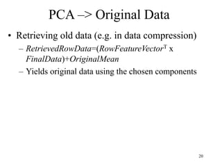
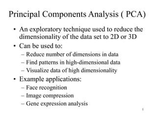
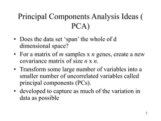
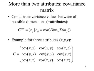
Principal Components Analysis (PCA) is an exploratory technique used to reduce the dimensionality of data sets while retaining as much information as possible. It transforms a number of correlated variables into a smaller number of uncorrelated variables called principal components. PCA is commonly used for applications like face recognition, image compression, and gene expression analysis by reducing the dimensions of large data sets and finding patterns in the data.

1. 1
Principal Components Analysis ( PCA)
• An exploratory technique used to reduce the
dimensionality of the data set to 2D or 3D
• Can be used to:
– Reduce number of dimensions in data
– Find patterns in high-dimensional data
– Visualize data of high dimensionality
• Example applications:
– Face recognition
– Image compression
– Gene expression analysis

2. 2
Principal Components Analysis Ideas (
PCA)
• Does the data set ‘span’ the whole of d
dimensional space?
• For a matrix of m samples x n genes, create a new
covariance matrix of size n x n.
• Transform some large number of variables into a
smaller number of uncorrelated variables called
principal components (PCs).
• developed to capture as much of the variation in
data as possible

3. 3
X1
X2
Principal Component Analysis
See online tutorials such as
http://www.cs.otago.ac.nz/cosc453/student_
tutorials/principal_components.pdf
Note: Y1 is
the first
eigen vector,
Y2 is the
second. Y2
ignorable.
Y1
Y2
x
x
x x
x
x
x
x
x
x
x
x
x x
x
x
x
x
x x
x
x
x
x
x
Key observation:
variance = largest!

4. 4
Principal Component Analysis: one
attribute first
• Question: how much
spread is in the data
along the axis?
(distance to the mean)
• Variance=Standard
deviation^2
Temperature
42
40
24
30
15
18
15
30
15
30
35
30
40
30
)
1
(
)
(
1
2
2





n
X
X
s
n
i
i

5. 5
Now consider two dimensions
X=Temperature Y=Humidity
40 90
40 90
40 90
30 90
15 70
15 70
15 70
30 90
15 70
30 70
30 70
30 90
40 70
)
1
(
)
)(
(
)
,
cov( 1






n
Y
Y
X
X
Y
X
n
i
i
i
Covariance: measures the
correlation between X and Y
• cov(X,Y)=0: independent
•Cov(X,Y)>0: move same dir
•Cov(X,Y)<0: move oppo dir

6. 6
More than two attributes: covariance
matrix
• Contains covariance values between all
possible dimensions (=attributes):
• Example for three attributes (x,y,z):
))
,
cov(
|
( j
i
ij
ij
nxn
Dim
Dim
c
c
C 












)
,
cov(
)
,
cov(
)
,
cov(
)
,
cov(
)
,
cov(
)
,
cov(
)
,
cov(
)
,
cov(
)
,
cov(
z
z
y
z
x
z
z
y
y
y
x
y
z
x
y
x
x
x
C

7. 7
Eigenvalues & eigenvectors
• Vectors x having same direction as Ax are called
eigenvectors of A (A is an n by n matrix).
• In the equation Ax=x,  is called an eigenvalue of A.


































2
3
4
8
12
2
3
1
2
3
2
x
x

8. 8
Eigenvalues & eigenvectors
• Ax=x  (A-I)x=0
• How to calculate x and :
– Calculate det(A-I), yields a polynomial
(degree n)
– Determine roots to det(A-I)=0, roots are
eigenvalues 
– Solve (A- I) x=0 for each  to obtain
eigenvectors x

9. 9
Principal components
• 1. principal component (PC1)
– The eigenvalue with the largest absolute value will
indicate that the data have the largest variance
along its eigenvector, the direction along which
there is greatest variation
• 2. principal component (PC2)
– the direction with maximum variation left in data,
orthogonal to the 1. PC
• In general, only few directions manage to
capture most of the variability in the data.

10. 10
Steps of PCA
• Let be the mean
vector (taking the mean
of all rows)
• Adjust the original data
by the mean
X’ = X –
• Compute the
covariance matrix C of
adjusted X
• Find the eigenvectors
and eigenvalues of C.
X
• For matrix C, vectors e
(=column vector) having
same direction as Ce :
– eigenvectors of C is e such
that Ce=e,
–  is called an eigenvalue of
C.
• Ce=e  (C-I)e=0
– Most data mining
packages do this for you.
X

11. 11
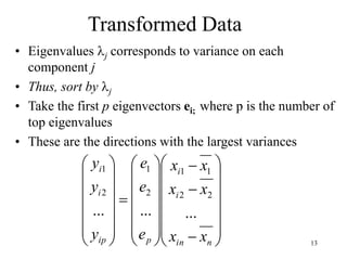
Eigenvalues
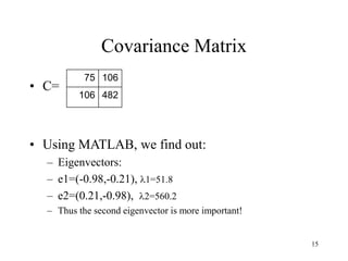
• Calculate eigenvalues  and eigenvectors x for
covariance matrix:
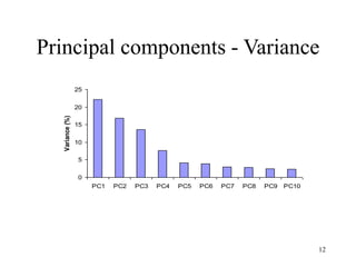
– Eigenvalues j are used for calculation of [% of total
variance] (Vj) for each component j:

 




n
x
x
n
x
x
j
j n
V
1
1
100 



12. 12
Principal components - Variance
0
5
10
15
20
25
PC1 PC2 PC3 PC4 PC5 PC6 PC7 PC8 PC9 PC10
Variance
(%)

13. 13
Transformed Data
• Eigenvalues j corresponds to variance on each
component j
• Thus, sort by j
• Take the first p eigenvectors ei; where p is the number of
top eigenvalues
• These are the directions with the largest variances














































n
in
i
i
p
ip
i
i
x
x
x
x
x
x
e
e
e
y
y
y
...
...
...
2
2
1
1
2
1
2
1

14. 14
An Example
X1 X2 X1' X2'
19 63 -5.1 9.25
39 74 14.9 20.25
30 87 5.9 33.25
30 23 5.9 -30.75
15 35 -9.1 -18.75
15 43 -9.1 -10.75
15 32 -9.1 -21.75
0
10
20
30
40
50
60
70
80
90
100
0 10 20 30 40 50
Series1
Mean1=24.1
Mean2=53.8
-40
-30
-20
-10
0
10
20
30
40
-15 -10 -5 0 5 10 15 20
Series1

15. 15
Covariance Matrix
• C=
• Using MATLAB, we find out:
– Eigenvectors:
– e1=(-0.98,-0.21), 1=51.8
– e2=(0.21,-0.98), 2=560.2
– Thus the second eigenvector is more important!
75 106
106 482

16. 16
If we only keep one dimension: e2
• We keep the dimension
of e2=(0.21,-0.98)
• We can obtain the final
data as
  2
1
2
1
*
98
.
0
*
21
.
0
98
.
0
21
.
0 i
i
i
i
i x
x
x
x
y 











-0.5
-0.4
-0.3
-0.2
-0.1
0
0.1
0.2
0.3
0.4
0.5
-40 -20 0 20 40
yi
-10.14
-16.72
-31.35
31.374
16.464
8.624
19.404
-17.63

17. 17

18. 18

19. 19

20. 20
PCA –> Original Data
• Retrieving old data (e.g. in data compression)
– RetrievedRowData=(RowFeatureVectorT x
FinalData)+OriginalMean
– Yields original data using the chosen components

21. 21
Principal components
• General about principal components
– summary variables
– linear combinations of the original variables
– uncorrelated with each other
– capture as much of the original variance as
possible

22. 22
Applications – Gene expression analysis
• Reference: Raychaudhuri et al. (2000)
• Purpose: Determine core set of conditions for useful
gene comparison
• Dimensions: conditions, observations: genes
• Yeast sporulation dataset (7 conditions, 6118 genes)
• Result: Two components capture most of variability
(90%)
• Issues: uneven data intervals, data dependencies
• PCA is common prior to clustering
• Crisp clustering questioned : genes may correlate with
multiple clusters
• Alternative: determination of gene’s closest neighbours

23. 23
Two Way (Angle) Data Analysis
Genes 103–104
Samples
10
1
-10
2
Gene expression
matrix
Sample space analysis Gene space analysis
Conditions 101–102
Genes
10
3
-10
4
Gene expression
matrix

24. 24
PCA - example

25. 25
PCA on all Genes
Leukemia data, precursor B and T
Plot of 34 patients, dimension of 8973 genes
reduced to 2

26. 26
PCA on 100 top significant genes
Leukemia data, precursor B and T
Plot of 34 patients, dimension of 100 genes
reduced to 2

27. 27
PCA of genes (Leukemia data)
Plot of 8973 genes, dimension of 34 patients reduced to 2