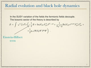
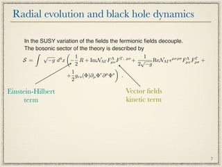
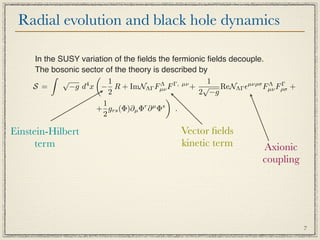
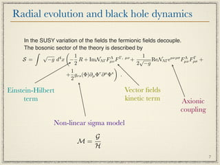
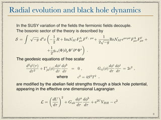
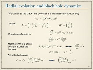
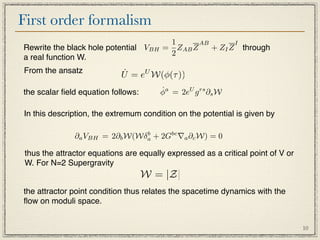
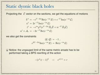
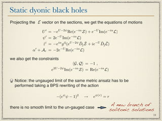
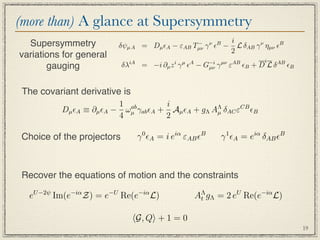
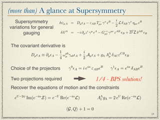
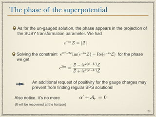
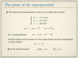
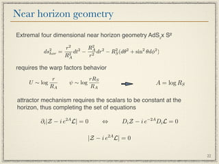
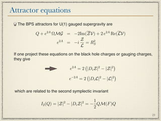
The document summarizes research on black hole solutions in gauged supergravity theories. It discusses how black holes in ungauged supergravity can be described using duality symmetries and extremality. For gauged supergravities, the addition of a scalar potential allows for asymptotically anti-de Sitter spacetimes. The dynamics of scalar fields near black hole horizons are governed by equations modified by gauge field strengths and an effective black hole potential. Specific examples are given in theories with one modulus and special Kähler geometries.

1. April 18th, 2011
Flow equations for AdS₄ black holes
in N=2 gauged supergravity
G. DallʼAgata, A.G. - arXiv:1012.3756
JHEP 1103:037,2011
Alessandra Gnecchi
“G. Galilei” Physics Dept. - Padua University (Italy)
& Dept. of Physics - Harvard University

2. Outline
Black holes in Supergravity
Duality invariance of extremal solutions
BPS flow of scalar fields
Black holes in gauged Supergravity
The FI gauging
One modulus and stu model examples
Future directions
2

3. Motivations
1. Gauged Supergravity
The low energy effective theories obtained from String Theory
compactifications in the presence of fluxes are gauged supergravities.
2. AdS space
The gauging appears as a scalar potential in the four dimensional action,
which plays the role of a coordinate dependent cosmological constant.
We seek a systematic approach to address the problem of
the destabilization of such backgrounds by the presence of
a stable black hole, thus yielding new insights into the
interpretation of string landscape.
3

4. Motivations
Other applications
1. Gauge/gravity duality
Not only the near horizon region develops an AdS geometry,
but also the asymptotic space!
2. AdS/CMT correspondence
Black holes solutions with scalars are associated to physical quantities in the
condensed matter system.
Building a solution with nontrivial scalar profiles, or
demonstrating the non existence in a specific models reflects
is a statement on the properties of the condensed matter
system
4

5. Black holes in Supergravity
Our approach:
Start from the formalism of un-gauged supergravity and exploit the
symmetries, in particular study theories with
electric-magnetic duality invariance
extremal black holes
Well established description in the last 15 years
S. Ferrara, R. Kallosh, A. Strominger hep-th/9508072
A. Strominger hep-th/9602111
S. Ferrara, G. W. Gibbons, R. Kallosh, hep-th/9702103
has lead to the classification of black hole charge orbits, multicenter solutions,
split attractors, wall crossing..
Cacciatori-Klemm 0911.4926: genuine black holes solutions with spherical
horizons in N=2 Supergravity with FI electric gauging.
5

6. Black holes in Supergravity
Describe regular solutions of the classical gravitational theory which are
stable:
no Hawking radiation but finite horizon area
they have zero temperature but finite entropy
extremal solutions
Already in 4d gravity, the Reissner Nordstrom solution has an extremal limit
r+ − r − κ 2
r+ − r− = 2 M 2 − Q2 κ= 2
2r+
T = →0 S= πr+
2π
In a gravity theory they saturates the bound M=|Q|
in a Supergravity theory the charge is substituted by the central charge,
and gives a BPS bound
M=|Z|
meaning the solution preserves some SUSY.
6

7. Radial evolution and black hole dynamics
In the SUSY variation of the fields the fermionic fields decouple.
The bosonic sector of the theory is described by
√ 1 1
S = −g d x − R + ImNΛΓ Fµν F
4 Λ Γ, µν
+ √ ReNΛΓ µνρσ Fµν Fρσ +
Λ Γ
2 2 −g
1
+ grs (Φ)∂µ Φr ∂ µ Φs .
2
7

8. Radial evolution and black hole dynamics
In the SUSY variation of the fields the fermionic fields decouple.
The bosonic sector of the theory is described by
√ 1 1
S = −g d x − R + ImNΛΓ Fµν F
4 Λ Γ, µν
+ √ ReNΛΓ µνρσ Fµν Fρσ +
Λ Γ
2 2 −g
1
+ grs (Φ)∂µ Φr ∂ µ Φs .
2
Einstein-Hilbert
term
7

9. Radial evolution and black hole dynamics
In the SUSY variation of the fields the fermionic fields decouple.
The bosonic sector of the theory is described by
√ 1 1
S = −g d x − R + ImNΛΓ Fµν F
4 Λ Γ, µν
+ √ ReNΛΓ µνρσ Fµν Fρσ +
Λ Γ
2 2 −g
1
+ grs (Φ)∂µ Φr ∂ µ Φs .
2
Einstein-Hilbert Vector fields
term kinetic term
7

10. Radial evolution and black hole dynamics
In the SUSY variation of the fields the fermionic fields decouple.
The bosonic sector of the theory is described by
√ 1 1
S = −g d x − R + ImNΛΓ Fµν F
4 Λ Γ, µν
+ √ ReNΛΓ µνρσ Fµν Fρσ +
Λ Γ
2 2 −g
1
+ grs (Φ)∂µ Φr ∂ µ Φs .
2
Einstein-Hilbert Vector fields
term kinetic term Axionic
coupling
7

11. Radial evolution and black hole dynamics
In the SUSY variation of the fields the fermionic fields decouple.
The bosonic sector of the theory is described by
√ 1 1
S = −g d x − R + ImNΛΓ Fµν F
4 Λ Γ, µν
+ √ ReNΛΓ µνρσ Fµν Fρσ +
Λ Γ
2 2 −g
1
+ grs (Φ)∂µ Φr ∂ µ Φs .
2
Einstein-Hilbert Vector fields
term kinetic term Axionic
coupling
Non-linear sigma model
G
M=
H
7

12. Radial evolution and black hole dynamics
In the SUSY variation of the fields the fermionic fields decouple.
The bosonic sector of the theory is described by
√ 1 1
S = −g d x − R + ImNΛΓ Fµν F
4 Λ Γ, µν
+ √ ReNΛΓ µνρσ Fµν Fρσ +
Λ Γ
2 2 −g
1
+ grs (Φ)∂µ Φr ∂ µ Φs .
2
The geodesic equations of free scalar
d2 φi (τ ) dφj dφk dφi dφj
i
+ Γjk (φ) = 0, Gij (φ) = 2c2 ,
dτ 2 dτ dτ dτ dτ
where c2 = 4S 2 T 2 .
are modified by the abelian field strengths through a black hole potential,
appearing in the effective one dimensional Lagrangian
2
dU dφa dφb
L= + Gab + e2U VBH − c2
dτ dτ dτ
8

13. Radial evolution and black hole dynamics
We can write the black hole potential in a manifestly symplectic way
1 TΛ
VBH = Q MΛΣ QΣ ,
2
Λ
where µ + νµ ν νµ
−1 −1
p
M = . Q =
Λ
,
µ−1 ν µ−1 qΛ
d2 U
= 2e2U VBH (φ, p, q),
Equations of motions: dτ 2
D2 φa 2U ∂VBH
2
= e a
,
Dτ ∂φ
Regularity of the scalar dφa
configuration at the Gij ∂m φi ∂n φj γ mn ∞ =0
dω
horizon: 1
ω = log ρ , ρ=− ,
τ
Attractor behaviour:
2π ∂VBH ∂VBH
a
φ ≈ φa
H + log τ =0
A ∂φa ∂φa hor
9

14. First order formalism
1 AB I
Rewrite the black hole potential VBH = ZAB Z + ZI Z through
2
a real function W.
From the ansatz ˙
U = eU W(φ(τ ))
the scalar field equation follows: ˙
φa = 2eU g rs ∂s W
In this description, the extremum condition on the potential is given by
∂a VBH = 2∂b W(Wδa + 2Gbc ∇a ∂c W) = 0
b
thus the attractor equations are equally expressed as a critical point of V or
W. For N=2 Supergravity
W = |Z|
the attractor point condition thus relates the spacetime dynamics with the
flow on moduli space.
10

15. BPS flow, rotating and non SUSY solutions
Extension to rotating solution [Denef, hep-th/0005049]
Exemples of multicenter configurations
N
¯ ω ¯
F, V = −e2iα [ζ + i (˜ ∧ ζ)] ζ= Z(Qi )dτi
i=1
Attractor equations describe also extremal, non supersymmetric black holes,
that can be built as intersecting branes systems from type IIA string theory
[Kallosh-Sivanandam-Soroush, hep-th/0602005]
[Gimon-Larsen-Simon, 0710.4967]
The first order description generalizes to the non-BPS case by introducing a
fake superpotential , built out of invariants of symplectic geometry
[Ceresole-DallʼAgata hep-th/0702088]
Extremal non-BPS solutions can be decomposed as threshold states of BPS
constituents, thus revealing the existence of multicenter extremal non
supersymmetric configurations, that one has to take into account when
counting the degeneracy of the black holes states.
[Gimon-Larsen-Simon, 0903.0719]
[Bena-DallʼAgata-Giusto-Ruef-Warner, 0902.4526]
11

16. The gauging
Momentum map procedure [Ceresole-DʼAuria-Ferrara, hep-th/9509160]
Let gi¯ be the Kähler metric of a Kähler manifold M. If it has a

a non trivial group of continuous isometries G generated by
Killing vectors, then the kinetic Lagrangian admits G as a
group of global space-time symmetries.
The holomorphic Killing vectors, which are defined by the
variation of the fields δz i = Λ kΛ (z) are defined by the
i
equations
∇i kj + ∇j ki = 0 ; ∇¯kj + ∇j k¯ = 0
ı ı
This are identically satisfied once we can write
kΛ = ig i¯∂¯PΛ ,
i 
 PΛ = PΛ
∗
thus defining a momentum map, which also preserves the
Kähler structure of the scalar manifold.
The momentum map construction applies to all manifolds with
a symplectic structure, in particular to Kähler, HyperKähler
and Quaternionic manifolds.
12

17. The gauging
[Ceresole-DʼAuria-Ferrara ʻ95]
Gauging involving hypermultiplets:
Triholomorphic momentum map that leaves invariant the
hyperkahler structure up to SU(2) rotations.
In N=2 theories the same group of isometries G acts both on
the SpecialKähler and HyperKähler manifolds:
ˆ
Λ = k i ∂i + k¯ ∂¯ + k u ∂u
ı
k Λ Λ ı Λ
Fayet-Iliopoulos gauging = constant prepotential
PΛ = ξΛ
x x
13

18. The gauging
[Ceresole-DʼAuria-Ferrara ʻ95]
Gauging involving hypermultiplets:
Triholomorphic momentum map that leaves invariant the
hyperkahler structure up to SU(2) rotations.
In N=2 theories the same group of isometries G acts both on
the SpecialKähler and HyperKähler manifolds:
ˆ
Λ = k i ∂i + k¯ ∂¯ + k u ∂u
ı
k Λ Λ ı Λ
Fayet-Iliopoulos gauging = constant prepotential
PΛ = ξΛ
x x
13

19. The gauging
[Ceresole-DʼAuria-Ferrara ʻ95]
Gauging involving hypermultiplets:
Triholomorphic momentum map that leaves invariant the
hyperkahler structure up to SU(2) rotations.
In N=2 theories the same group of isometries G acts both on
the SpecialKähler and HyperKähler manifolds:
ˆ
Λ = k i ∂i + k¯ ∂¯ + k u ∂u
ı
k Λ Λ ı Λ
Fayet-Iliopoulos gauging = constant prepotential
PΛ = ξΛ
x x
Non-trivial gauging!
13

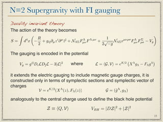
20. N=2 Supergravity with FI gauging
[Ceresole-DʼAuria-Ferrara ʻ95]
Consider the scalar potential for an N=2 theory.
Due to the fact that all the relevant quantities are derived from
the Kähler vectors and prepotential, this can be written in a
geometrical way as
¯ ¯
V = (kΛ , kΣ )LΛ LΣ + (U ΛΣ − 3LΛ LΣ )(PΛ PΣ − PΛ PΣ )
x x
Thus, one easily sees that for an abelian theory this potential
can still be nonzero, as long as the prepotentials are taken as
constants, PΛ = ξΛ leading to the form of V on which we will
x x
focus:
VF I = (U ΛΣ ¯ Λ LΣ )ξΛ ξΣ
− 3L x x
14

21. N=2 Supergravity with FI gauging
Duality invariant theory
The action of the theory becomes
R 1
S= d x − + gi¯∂µ z ∂ z + NΛΣ Fµν F
4
 ¯
i µ ¯
 Λ Λ µν
+ √ NΛΣ µνρσ Fµν Fρσ − Vg
Λ Σ
2 2 −g
The gauging is encoded in the potential
Vg = g Di LD¯L − 3|L|
i¯


2
where L = G, V = eK/2 Λ
X gΛ − FΛ g Λ
it extends the electric gauging to include magnetic gauge charges, it is
constructed only in terms of symplectic sections and symplectic vector of
charges
V = eK/2 (X Λ (z), FΛ (z)) G = (˜Λ , gΛ )
g
analogously to the central charge used to define the black hole potential
Z ≡ Q, V VBH = |DZ|2 + |Z|2
15

22. Static dyonic black holes
Ansatz for the space-time background
ds2 = −e2U (r) dt2 + e−2U (r) (dr2 + e2ψ(r) dΩ2 )
A second warp factor provides the deviation from the ansatz for
asymptotically flat configurations.
It compensates for the additional contribution to Einstein equations
due to the non-trivial cosmological constant.
In general the existence of BPS solutions only constrains the three
dimensional base to be a space
ds2 = dz 2 + e2Φ dwdw
3 ¯
with U(1) holonomy and torsion.
16

23. Static dyonic black holes
The effective action for a static spherically configuration becomes
2ψ 2 2 i 
¯ 2U −4ψ −2U
S1d = dr e U − ψ + gi¯z z + e
 ¯ VBH + e Vg − 1
d 2ψ
+ dr e (2ψ − U )
dr
17

24. Static dyonic black holes
The effective action for a static spherically configuration becomes
2ψ 2 2 i 
¯ 2U −4ψ −2U
S1d = dr e U − ψ + gi¯z z + e
 ¯ VBH + e Vg − 1
d 2ψ
+ dr e (2ψ − U )
dr
Possible squaring?
17

25. Static dyonic black holes
The effective action for a static spherically configuration becomes
2ψ 2 2 i 
¯ 2U −4ψ −2U
S1d = dr e U − ψ + gi¯z z + e
 ¯ VBH + e Vg − 1
d 2ψ
+ dr e (2ψ − U )
dr
17

26. Static dyonic black holes
The effective action for a static spherically configuration becomes
2ψ 2 2 i 
¯ 2U −4ψ −2U
S1d = dr e U − ψ + gi¯z z + e
 ¯ VBH + e Vg − 1
d 2ψ
+ dr e (2ψ − U )
dr
The same action can be written
1 2(U −ψ) T 2ψ
−U −iα
2
S1d = dr − e E ME − e (α + Ar ) + 2e Re(e L)
2
2ψ
−U −iα
2
−e ψ − 2e Im(e L) − (1 + G, Q)
d 2ψ−U −iα U −iα
−2 e Im(e L) + e Re(e Z)
dr
this, together with
−U −iα
T
E ≡ 2e 2ψ
e Im(e V) T
− e2(ψ−U ) G T ΩM−1 + 4e−U (α + Ar )Re(e−iα V)T + QT
gives the BPS equations
17

27. Static dyonic black holes
Projecting the E vector on the sections, we get the equations of motions
U = −eU −2ψ Re(e−iα Z) + e−U Im(e−iα L)
ψ = 2e−U Im(e−iα L)
¯ ¯ ¯ ¯
z i = −eiα g i¯(eU −2ψ D¯Z + ie−U D¯L)
˙ 
α + Ar = −2e−U Re(e−iα L)
we also get the constraints
G, Q = −1 ,
e2U −2ψ Im(e−iα Z) = Re(e−iα L)
Notice: the ungauged limit of the same metric ansatz has to be
performed taking a BPS rewriting of the action
−(eψ ψ − 1)2 → eψ(r) = r
18

28. Static dyonic black holes
Projecting the E vector on the sections, we get the equations of motions
U = −eU −2ψ Re(e−iα Z) + e−U Im(e−iα L)
ψ = 2e−U Im(e−iα L)
¯ ¯ ¯ ¯
z i = −eiα g i¯(eU −2ψ D¯Z + ie−U D¯L)
˙ 
α + Ar = −2e−U Re(e−iα L)
we also get the constraints
G, Q = −1 ,
e2U −2ψ Im(e−iα Z) = Re(e−iα L)
Notice: the ungauged limit of the same metric ansatz has to be
performed taking a BPS rewriting of the action
−(eψ ψ − 1)2 → eψ(r) = r
A new branch of
there is no smooth limit to the un-gauged case
solitonic solutions
18

29. (more than) A glance at Supersymmetry
Supersymmetry − i
δψµ A = Dµ A − εAB Tµν γ − L δAB γ ν ηµν B
ν B
2
variations for general
i
gauging δλiA = −i ∂µ z i γ µ A − G−i γ µν εAB B + D L δ AB B
µν
The covariant derivative is
1 ab i
Dµ A ≡ ∂µ A − ωµ γab A + Aµ A + gΛ AΛ δAC εCB B
µ
4 2
Choice of the projectors γ 0 A = i eiα εAB B γ 1 A = eiα δAB B
Recover the equations of motion and the constraints
eU −2ψ Im(e−iα Z) = e−U Re(e−iα L) AΛ gΛ = 2 eU Re(e−iα L)
t
G, Q + 1 = 0
19

30. (more than) A glance at Supersymmetry
Supersymmetry − i
δψµ A = Dµ A − εAB Tµν γ − L δAB γ ν ηµν B
ν B
2
variations for general
i
gauging δλiA = −i ∂µ z i γ µ A − G−i γ µν εAB B + D L δ AB B
µν
The covariant derivative is
1 ab i
Dµ A ≡ ∂µ A − ωµ γab A + Aµ A + gΛ AΛ δAC εCB B
µ
4 2
Choice of the projectors γ 0 A = i eiα εAB B γ 1 A = eiα δAB B
Two projections required 1/4 - BPS solutions!
Recover the equations of motion and the constraints
eU −2ψ Im(e−iα Z) = e−U Re(e−iα L) AΛ gΛ = 2 eU Re(e−iα L)
t
G, Q + 1 = 0
19

31. The phase of the superpotential
As for the un-gauged solution, the phase appears in the projection of
the SUSY transformation parameter. We had
e−iα Z = |Z|
Solving the constraint e2U −2ψ Im(e−iα Z) = Re(e−iα L) for the phase
we get
Z − ie2(ψ−U ) L
e2iα = ¯ ¯
Z + ie2(ψ−U ) L
An additional request of positivity for the gauge charges may
prevent from finding regular BPS solutions!
Also notice, itʼs no more α + Ar = 0
(It will be recovered at the horizon)
20

32. The phase of the superpotential
The flow can be expressed in terms of a single real function

 U = −g U U ∂U W
ψ = −g ψψ ∂ψ W

z i = −2˜i¯∂¯W
˙ g 
gU U = −gψψ = e2ψ , gi¯ = e2ψ gi¯
˜ 
for a superpotential W = eU |Z − ie2(ψ−U ) L|
the flow stops at the horizon for the scalar fields and the combination
of warp factors
A=ψ−U
At the attractor point ∂i W|h = 0 , W|h = 0
21

33. Near horizon geometry
Extremal four dimensional near horizon geometry AdS₂x S²
r 2 2 RA 2
2
ds2
hor = 2 dt − 2 dr − RS (dθ2 + sin2 θdφ2 )
2
RA r
requires the warp factors behavior
r rRS
U ∼ log ψ ∼ log A = log RS
RA RA
attractor mechanism requires the scalars to be constant at the
horizon, thus completing the set of equations
∂i |Z − i e2A L| = 0 ⇔ Di Z − i e−2A Di L = 0
|Z − i e2A L| = 0
22

34. Attractor equations
The BPS attractors for U(1) gauged supergravity are
Q + e2A ΩMG = −2Im(ZV) + 2 e2A Re(LV)
2A Z 2
e = −i = RS
L
If one project these equations on the black hole charges or gauging charges,
they give
2A
2 2
e = 2 |Di Z| − |Z|
−2A
2 2
e = 2 |Di L| − |L|
which are related to the second symplectic invariant
2 2 1
I2 (Q) = |Z| − |Di Z| = − QM(F )Q
2
23

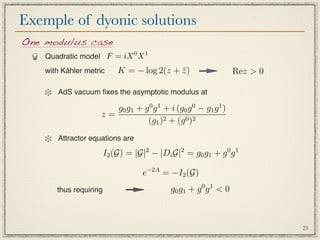
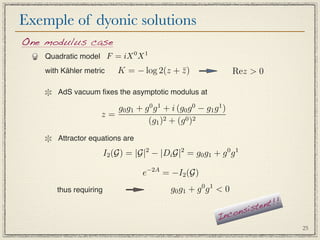
35. Solutions with constant scalars
Asymptotic AdS background : Di L = 0
Equal radii would imply vanishing potential at the horizon
R S = RA → Vg = 0 [Bellucci-Ferrara-Marrani-Yeranyan ʻ08]
The form of the gauge potential: Vg = −3|L|2 + |DL|2
A configuration with constant scalars along the flow has |L| = 0
In general, for constant scalars, the attractor equations imply
2A Im(ZL) 2A 1 G, Q
e =− e =
|L|2 2 |L|2
which is inconsistent for spherical horizons for which G, Q = −1 0
24

36. Exemple of dyonic solutions
One modulus case
Quadratic model F = iX 0 X 1
with Kähler metric K = − log 2(z + z )
¯ Rez 0
AdS vacuum fixes the asymptotic modulus at
g0 g1 + g 0 g 1 + i (g0 g 0 − g1 g 1 )
z=
(g1 )2 + (g 0 )2
Attractor equations are
I2 (G) = |G|2 − |Di G|2 = g0 g1 + g 0 g 1
e−2A = −I2 (G)
thus requiring g0 g1 + g 0 g 1 0
25

37. Exemple of dyonic solutions
One modulus case
Quadratic model F = iX 0 X 1
with Kähler metric K = − log 2(z + z )
¯ Rez 0
AdS vacuum fixes the asymptotic modulus at
g0 g1 + g 0 g 1 + i (g0 g 0 − g1 g 1 )
z=
(g1 )2 + (g 0 )2
Attractor equations are
I2 (G) = |G|2 − |Di G|2 = g0 g1 + g 0 g 1
e−2A = −I2 (G)
thus requiring g0 g1 + g 0 g 1 0
!!
sis tent
I ncon
25

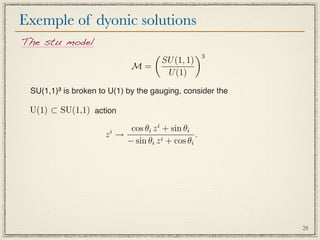
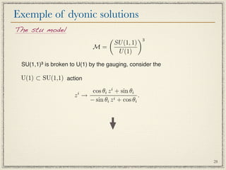
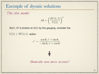
38. Exemple of dyonic solutions
The stu model
X 1X 2X 3
STU model with prepotential F =− : the potential of the
X0
gauging has no critical point no asymptotic AdS configurations.
√
STU model with prepotential F = −i X 0 X 1 X 2 X 3 admits regular
solutions with spherical horizon for magnetic charges
[Cacciatori-Klemm 0911.4926]
the duality invariant setup allow us to build a genuine dyonic
solution by rotation of both electromagnetic and gauging charges
VCK = eK/2 (1, −tu, −su, −st, −stu, s, t, u)T  
1
K/2 T  −1 
V=e (1, s, t, u, −stu, tu, su, st) 
 −1


 
 −1 
S=



 1 
 
VCK = SV G = S −1 GCK 

1
1


−1 1
Q = S QCK
26

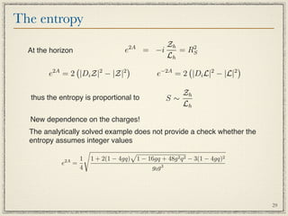
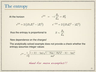
39. Exemple of dyonic solutions
The stu model Charges
Kahler potential Q = (p0 , 0, 0, 0, 0, q1 , q2 , q3 )T
¯ ¯
K = − log[−i(s − s)(t − t)(u − u)]
¯ G = (0, g 1 , g 2 , g 3 , g0 , 0, 0, 0)T
Superpotential
W = eK/2 |q1 s + q2 t + q3 u + p0 stu − ie2A (g0 − g 1 tu − g 2 su − g 3 st)|
No axion solution Re s = Re t = Re u = 0
The case where all the scalars are identified can be solved analitically;
the attractor values of the fields are
g0 −1 + 6gq + 1 − 16gq + 48g 2 q 2
y= 0
2g 1 − 3gq
2A 1 1 + 2(1 − 4gq) 1 − 16gq + 48g 2 q 2 − 3(1 − 4gq)2
e =
4 g0 g 3
27

40. Exemple of dyonic solutions
The stu model
3
SU (1, 1)
M=
U (1)
SU(1,1)³ is broken to U(1) by the gauging, consider the
U(1) ⊂ SU(1,1) action
cos θi z i + sin θi
zi → i + cos θ
.
− sin θi z i
28

41. Exemple of dyonic solutions
The stu model
3
SU (1, 1)
M=
U (1)
SU(1,1)³ is broken to U(1) by the gauging, consider the
U(1) ⊂ SU(1,1) action
cos θi z i + sin θi
zi → i + cos θ
.
− sin θi z i
28

42. Exemple of dyonic solutions
The stu model
3
SU (1, 1)
M=
U (1)
SU(1,1)³ is broken to U(1) by the gauging, consider the
U(1) ⊂ SU(1,1) action
cos θi z i + sin θi
zi → i + cos θ
.
− sin θi z i
Generate non zero axions!
28

43. The entropy
2A Zh 2
At the horizon e = −i = RS
Lh
2A
2 2
−2A
2 2
e = 2 |Di Z| − |Z| e = 2 |Di L| − |L|
Zh
thus the entropy is proportional to S∼
Lh
New dependence on the charges!
The analytically solved example does not provide a check whether the
entropy assumes integer values
2A 1 1 + 2(1 − 4gq) 1 − 16gq + 48g 2 q 2 − 3(1 − 4gq)2
e =
4 g0 g 3
29

44. The entropy
2A Zh 2
At the horizon e = −i = RS
Lh
2A
2 2
−2A
2 2
e = 2 |Di Z| − |Z| e = 2 |Di L| − |L|
Zh
thus the entropy is proportional to S∼
Lh
New dependence on the charges!
The analytically solved example does not provide a check whether the
entropy assumes integer values
2A 1 1 + 2(1 − 4gq) 1 − 16gq + 48g 2 q 2 − 3(1 − 4gq)2
e =
4 g0 g 3
Need for more examples!!
29

45. Future developments 1. Flow equations
What’s the geometric meaning of the gauging?
Multiplying by the symplectic operator MΩ + i ,
the attractor equations can be expanded to give
−iα −U
2A
Q + e ΩMG = −2e 2A+2U
Im −iα −U
∂r + i(α + Ar − 2Re(e
˙ e L)) (e e V)
confront them with the un-gauged flow
−iα −U
Q = −2Im (∂r + i(α + Ar ) (e e V)
˙
Need for an interpretation of the “gauging section”
What happens to the harmonic functions?
30

46. Future developments 1. Flow equations
What’s the geometric meaning of the gauging?
Multiplying by the symplectic operator MΩ + i ,
the attractor equations can be expanded to give
−iα −U
2A
Q + e ΩMG = −2e 2A+2U
Im −iα −U
∂r + i(α + Ar − 2Re(e
˙ e L)) (e e V)
confront them with the un-gauged flow
−iα −U
Q = −2Im (∂r + i(α + Ar ) (e e V)
˙
Need for an interpretation of the “gauging section”
What happens to the harmonic functions?
Possible insights from a higher dimensional construction!
30

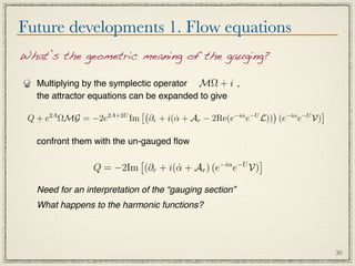
47. Future developments 2. M-theory embedding
Reductions from 10 or 11 dimensions on spheres preserve to many
supersymmetries.
Additional truncations are possible, leading to N=2 U(1) gauged
supergravity
[Cvetič-Duff-Hoxha-Liu-Lü-Lu-Martinez Acosta-Pope-
Sati-Tran, hep-th/9903214]
M-theory reductions give in this cases only magnetic charges
The magnetic field mixes internal angles and 4dim angular variables.
This would require the presence of topological charges in the low
energy configuration, but such monopoles might break all the
supersymmetries [Vandoren-Hristov, 1012.4314]
31

48. Future developments 3. Rotating BHs
D. Klemm arxiv:1103.4699, the solutions have an enhancement of
supersymmetry at the horizon: 1/2-BPS black holes
How does the attractor equations get
modified for these solutions?
The metric ansatz in the rotating case can be modified introducing the
fibration
ds2 = −e2U (dt + ω)2 + e−2U (dr2 + e−2ψ dΩ2 )
keeping the three base space conformally flat
do multicenter solutions also exist?
Does the generalization of the symplectic section defining the
prepotential govern the dynamics in the rotating case?
32

49. Future developments
4. More general gaugings - Adding Hypermultiplets
Hypermultiplets are always present in theories obtained from flux
compactifications
Gauging of non-abelian isometries requires nontrivial scalar charge,
what happens to the attractor mechanism?
5. Extend these solutions out of extremality
Duff-Liu, hep-th/9901149: “merging” of the gauging and the out-of-
extremality contribution in metric functions
dr2
ds2 = −e2A f dt2 + e2B ( + r2 dΩ2 )
f
k 2 2
f = 1 − + 2g r (H1 H2 H3 H4 )
r
Interesting phenomena might be described from an holographic
perpective, once the finite temperature system is known.
33

50. Conclusions
Asymptotically non flat solutions have been studied using the
geometric formulation of duality invariant supergravities.
Very close analogies have been found to the un-gauged case, and an
easy generalization obtained for the superpotential of N=2
supergravity
Although in the standard lore static and supersymmetric solutions are
singular, many regular solutions are found, representing a new
solitonic branch, for charges satisfying the constraint
G, Q = −1
There is however an incomplete enhancement of SUSY at the
horizon: 1/4-BPS solutions.
34

51. Conclusions
Asymptotically non flat solutions have been studied using the
geometric formulation of duality invariant supergravities.
Very close analogies have been found to the un-gauged case, and an
easy generalization obtained for the superpotential of N=2
supergravity
Although in the standard lore static and supersymmetric solutions are
singular, many regular solutions are found, representing a new
solitonic branch, for charges satisfying the constraint
G, Q = −1
There is however an incomplete enhancement of SUSY at the
horizon: 1/4-BPS solutions.
Definitely more to come!
34