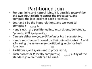
This document discusses parallel databases and different types of parallelism that can be utilized in databases including I/O parallelism, interquery parallelism, intraquery parallelism, and interoperation parallelism. It provides details on how relations can be partitioned across multiple disks for I/O parallelism using techniques like round robin, hash partitioning, and range partitioning. It also compares these partitioning techniques in terms of supporting full relation scans, point queries, and range queries.

1. UNIT-1
Parallel Databases
ADBMS-UNIT-1 1

2. Chapter 1: Parallel Databases
• Introduction
• I/O Parallelism
• Interquery Parallelism
• Intraquery Parallelism
• Intraoperation Parallelism
• Interoperation Parallelism
• Design of Parallel Systems
ADBMS-UNIT-1 2

3. Introduction
• Parallel machines are becoming quite common and
affordable
– Prices of microprocessors, memory and disks have
dropped sharply
– Recent desktop computers feature multiple
processors and this trend is projected to accelerate
• Databases are growing increasingly large
– large volumes of transaction data are collected and
stored for later analysis.
– multimedia objects like images are increasingly stored
in databases
• Large-scale parallel database systems increasingly
used for:
– storing large volumes of data
– processing time-consuming decision-support queries
– providing high throughput for transaction processing
ADBMS-UNIT-1 3

4. Parallelism in Databases
• Data can be partitioned across multiple disks for parallel
I/O.
• Individual relational operations (e.g., sort, join,
aggregation) can be executed in parallel
– data can be partitioned and each processor can work
independently on its own partition.
• Queries are expressed in high level language (SQL,
translated to relational algebra)
– makes parallelization easier.
• Different queries can be run in parallel with each other.
Concurrency control takes care of conflicts.
• Thus, databases naturally lend themselves to parallelism.
ADBMS-UNIT-1 4

5. I/O Parallelism
• Reduce the time required to retrieve relations from disk by
partitioning
• the relations on multiple disks.
• Horizontal partitioning – tuples of a relation are divided
among many disks such that each tuple resides on one disk.
• Partitioning techniques (number of disks = n):
Round-robin:
Send the ith tuple inserted in the relation to disk i mod n.
Hash partitioning:
– Choose one or more attributes as the partitioning attributes.
– Choose hash function h with range 0…n - 1
– Let i denote result of hash function h applied to the partitioning
attribute value of a tuple. Send tuple to disk i.
ADBMS-UNIT-1 5

6. I/O Parallelism (Cont.)
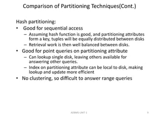
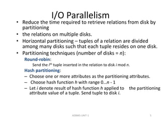
• Partitioning techniques (cont.):
• Range partitioning:
– Choose an attribute as the partitioning attribute.
– A partitioning vector [vo, v1, ..., vn-2] is chosen.
– Let v be the partitioning attribute value of a tuple.
Tuples such that vi  vi+1 go to disk I + 1. Tuples with v
< v0 go to disk 0 and tuples with v  vn-2 go to disk n-1.
E.g., with a partitioning vector [5,11], a tuple with
partitioning attribute value of 2 will go to disk 0, a
tuple with value 8 will go to disk 1, while a tuple with
value 20 will go to disk2.
ADBMS-UNIT-1 6

7. Comparison of Partitioning Techniques
• Evaluate how well partitioning techniques
support the following types of data access:
1.Scanning the entire relation.
2.Locating a tuple associatively – point queries.
– E.g., r.A = 25.
3.Locating all tuples such that the value of a given
attribute lies within a specified range – range
queries.
– E.g., 10  r.A < 25.
ADBMS-UNIT-1 7

8. Comparison of Partitioning Techniques (Cont.)
Round robin:
• Advantages
– Best suited for sequential scan of entire relation on
each query.
– All disks have almost an equal number of tuples;
retrieval work is thus well balanced between disks.
• Range queries are difficult to process
– No clustering -- tuples are scattered across all disks
ADBMS-UNIT-1 8

9. Comparison of Partitioning Techniques(Cont.)
Hash partitioning:
• Good for sequential access
– Assuming hash function is good, and partitioning attributes
form a key, tuples will be equally distributed between disks
– Retrieval work is then well balanced between disks.
• Good for point queries on partitioning attribute
– Can lookup single disk, leaving others available for
answering other queries.
– Index on partitioning attribute can be local to disk, making
lookup and update more efficient
• No clustering, so difficult to answer range queries
ADBMS-UNIT-1 9

10. Comparison of Partitioning Techniques (Cont.)
• Range partitioning:
• Provides data clustering by partitioning attribute value.
• Good for sequential access
• Good for point queries on partitioning attribute: only one disk
needs to be accessed.
• For range queries on partitioning attribute, one to a few disks
may need to be accessed
– Remaining disks are available for other queries.
– Good if result tuples are from one to a few blocks.
– If many blocks are to be fetched, they are still fetched from one to
a few disks, and potential parallelism in disk access is wasted
• Example of execution skew.
ADBMS-UNIT-1 10

11. Partitioning a Relation across Disks
• If a relation contains only a few tuples which will fit
into a single disk block, then assign the relation to
a single disk.
• Large relations are preferably partitioned across all
the available disks.
• If a relation consists of m disk blocks and there are
n disks available in the system, then the relation
should be allocated min(m,n) disks.
ADBMS-UNIT-1 11

12. Handling of Skew
• The distribution of tuples to disks may be skewed
— that is, some disks have many tuples, while
others may have fewer tuples.
• Types of skew:
– Attribute-value skew.
• Some values appear in the partitioning attributes of many
tuples; all the tuples with the same value for the partitioning
attribute end up in the same partition.
• Can occur with range-partitioning and hash-partitioning.
– Partition skew.
• With range-partitioning, badly chosen partition vector may
assign too many tuples to some partitions and too few to
others.
• Less likely with hash-partitioning if a good hash-function is
chosen.
ADBMS-UNIT-1 12

13. Handling Skew in Range-Partitioning
• To create a balanced partitioning vector (assuming
partitioning attribute forms a key of the relation):
– Sort the relation on the partitioning attribute.
– Construct the partition vector by scanning the relation in
sorted order as follows.
• After every 1/nth of the relation has been read, the value of the
partitioning attribute of the next tuple is added to the partition
vector.
– n denotes the number of partitions to be constructed.
– Duplicate entries or imbalances can result if duplicates
are present in partitioning attributes.
• Alternative technique based on histograms used in
practice
ADBMS-UNIT-1 13

14. Handling Skew using Histograms
 Balanced partitioning vector can be constructed from histogram in a relatively
straightforward fashion
 Assume uniform distribution within each range of the histogram
 Histogram can be constructed by scanning relation, or sampling (blocks containing)
tuples of the relation
ADBMS-UNIT-1 14

15. Handling Skew Using Virtual Processor
Partitioning
• Skew in range partitioning can be handled elegantly
using virtual processor partitioning:
– create a large number of partitions (say 10 to 20 times the
number of processors)
– Assign virtual processors to partitions either in round-robin
fashion or based on estimated cost of processing each
virtual partition
• Basic idea:
– If any normal partition would have been skewed, it is very
likely the skew is spread over a number of virtual partitions
– Skewed virtual partitions get spread across a number of
processors, so work gets distributed evenly!
ADBMS-UNIT-1 15

16. Interquery Parallelism
• Queries/transactions execute in parallel with one another.
• Increases transaction throughput; used primarily to scale up a
transaction processing system to support a larger number of
transactions per second.
• Easiest form of parallelism to support, particularly in a shared-memory
parallel database, because even sequential database
systems support concurrent processing.
• More complicated to implement on shared-disk or shared-nothing
architectures
– Locking and logging must be coordinated by passing messages
between processors.
– Data in a local buffer may have been updated at another processor.
– Cache-coherency has to be maintained — reads and writes of data
in buffer must find latest version of data.
ADBMS-UNIT-1 16

17. Cache Coherency Protocol
• Example of a cache coherency protocol for shared disk systems:
– Before reading/writing to a page, the page must be locked in
shared/exclusive mode.
– On locking a page, the page must be read from disk
– Before unlocking a page, the page must be written to disk if it was
modified.
• More complex protocols with fewer disk reads/writes exist.
• Cache coherency protocols for shared-nothing systems are
similar. Each database page is assigned a home processor.
Requests to fetch the page or write it to disk are sent to the
home processor.
ADBMS-UNIT-1 17

18. Intraquery Parallelism
• Execution of a single query in parallel on multiple
processors/disks; important for speeding up long-running
queries.
• Two complementary forms of intraquery parallelism :
– Intraoperation Parallelism – parallelize the execution of each
individual operation in the query.
– Interoperation Parallelism – execute the different operations in a
query expression in parallel.
the first form scales better with increasing parallelism because
the number of tuples processed by each operation is typically
more than the number of operations in a query
ADBMS-UNIT-1 18

19. Parallel Processing of Relational Operations
• Our discussion of parallel algorithms assumes:
– read-only queries
– shared-nothing architecture
– n processors, P0, ..., Pn-1, and n disks D0, ..., Dn-1, where disk
Di is associated with processor Pi.
• If a processor has multiple disks they can simply
simulate a single disk Di.
• Shared-nothing architectures can be efficiently
simulated on shared-memory and shared-disk systems.
– Algorithms for shared-nothing systems can thus be run on
shared-memory and shared-disk systems.
– However, some optimizations may be possible.
ADBMS-UNIT-1 19

20. Parallel Sort
Range-Partitioning Sort
• Choose processors P0, ..., Pm, where m  n -1 to do sorting.
• Create range-partition vector with m entries, on the sorting
attributes
• Redistribute the relation using range partitioning
– all tuples that lie in the ith range are sent to processor Pi
– Pi stores the tuples it received temporarily on disk Di.
– This step requires I/O and communication overhead.
• Each processor Pi sorts its partition of the relation locally.
• Each processors executes same operation (sort) in parallel with
other processors, without any interaction with the others (data
parallelism).
• Final merge operation is trivial: range-partitioning ensures that,
for 1 j m, the key values in processor Pi are all less than the key
values in Pj.
ADBMS-UNIT-1 20

21. Parallel Sort (Cont.)
Parallel External Sort-Merge
• Assume the relation has already been partitioned among
disks D0, ..., Dn-1 (in whatever manner).
• Each processor Pi locally sorts the data on disk Di.
• The sorted runs on each processor are then merged to get
the final sorted output.
• Parallelize the merging of sorted runs as follows:
– The sorted partitions at each processor Pi are range-partitioned
across the processors P0, ..., Pm-1.
– Each processor Pi performs a merge on the streams as they are
received, to get a single sorted run.
– The sorted runs on processors P0,..., Pm-1 are concatenated to
get the final result.
ADBMS-UNIT-1 21

22. Parallel Join
• The join operation requires pairs of tuples to be
tested to see if they satisfy the join condition, and
if they do, the pair is added to the join output.
• Parallel join algorithms attempt to split the pairs
to be tested over several processors. Each
processor then computes part of the join locally.
• In a final step, the results from each processor
can be collected together to produce the final
result.
ADBMS-UNIT-1 22

23. Partitioned Join
• For equi-joins and natural joins, it is possible to partition
the two input relations across the processors, and
compute the join locally at each processor.
• Let r and s be the input relations, and we want to
compute r r.A=s.B s.
• r and s each are partitioned into n partitions, denoted r0,
r1, ..., rn-1 and s0, s1, ..., sn-1.
• Can use either range partitioning or hash partitioning.
• r and s must be partitioned on their join attributes r.A and
s.B), using the same range-partitioning vector or hash
function.
• Partitions ri and si are sent to processor Pi,
• Each processor Pi locally computes ri ri.A=si.B si. Any of the
standard join methods can be used.
ADBMS-UNIT-1 23

24. Partitioned Join (Cont.)
ADBMS-UNIT-1 24

25. Fragment-and-Replicate Join
• Partitioning not possible for some join conditions
– e.g., non-equijoin conditions, such as r.A > s.B.
• For joins were partitioning is not applicable,
parallelization can be accomplished by fragment and
replicate technique
– Depicted on next slide
• Special case – asymmetric fragment-and-replicate:
– One of the relations, say r, is partitioned; any partitioning
technique can be used.
– The other relation, s, is replicated across all the processors.
– Processor Pi then locally computes the join of ri with all of s
using any join technique.
ADBMS-UNIT-1 25

26. Depiction of Fragment-and-Replicate Joins
ADBMS-UNIT-1f 26

27. Fragment-and-Replicate Join (Cont.)
• General case: reduces the sizes of the relations at each
processor.
– r is partitioned into n partitions,r0, r1, ..., r n-1;s is
partitioned into m partitions, s0, s1, ..., sm-1.
– Any partitioning technique may be used.
– There must be at least m * n processors.
– Label the processors as
– P0,0, P0,1, ..., P0,m-1, P1,0, ..., Pn-1m-1.
– Pi,j computes the join of ri with sj. In order to do so, ri is
replicated to Pi,0, Pi,1, ..., Pi,m-1, while si is replicated to P0,i,
P1,i, ..., Pn-1,i
– Any join technique can be used at each processor Pi,j.
ADBMS-UNIT-1 27

28. Fragment-and-Replicate Join (Cont.)
• Both versions of fragment-and-replicate work with any
join condition, since every tuple in r can be tested with
every tuple in s.
• Usually has a higher cost than partitioning, since one
of the relations (for asymmetric fragment-and-replicate)
or both relations (for general fragment-and-replicate)
have to be replicated.
• Sometimes asymmetric fragment-and-replicate is
preferable even though partitioning could be used.
– E.g., say s is small and r is large, and already partitioned. It
may be cheaper to replicate s across all processors, rather
than repartition r and s on the join attributes.
ADBMS-UNIT-1 28

29. Partitioned Parallel Hash-Join
Parallelizing partitioned hash join:
• Assume s is smaller than r and therefore s is chosen as the
build relation.
• A hash function h1 takes the join attribute value of each
tuple in s and maps this tuple to one of the n processors.
• Each processor Pi reads the tuples of s that are on its disk
Di, and sends each tuple to the appropriate processor
based on hash function h1. Let si denote the tuples of
relation s that are sent to processor Pi.
• As tuples of relation s are received at the destination
processors, they are partitioned further using another hash
function, h2, which is used to compute the hash-join locally.
(Cont.)
ADBMS-UNIT-1 29

30. Partitioned Parallel Hash-Join (Cont.)
• Once the tuples of s have been distributed, the larger relation r is
redistributed across the m processors using the hash function h1
– Let ri denote the tuples of relation r that are sent to processor Pi.
• As the r tuples are received at the destination processors, they are
repartitioned using the function h2
– (just as the probe relation is partitioned in the sequential hash-join
algorithm).
• Each processor Pi executes the build and probe phases of the hash-join
algorithm on the local partitions ri and s of r and s to produce a
partition of the final result of the hash-join.
• Note: Hash-join optimizations can be applied to the parallel case
– e.g., the hybrid hash-join algorithm can be used to cache some of the
incoming tuples in memory and avoid the cost of writing them and
reading them back in.
ADBMS-UNIT-1 30

31. Parallel Nested-Loop Join
• Assume that
– relation s is much smaller than relation r and that r is stored by
partitioning.
– there is an index on a join attribute of relation r at each of the
partitions of relation r.
• Use asymmetric fragment-and-replicate, with relation s being
replicated, and using the existing partitioning of relation r.
• Each processor Pj where a partition of relation s is stored reads the
tuples of relation s stored in Dj, and replicates the tuples to every
other processor Pi.
– At the end of this phase, relation s is replicated at all sites that store
tuples of relation r.
• Each processor Pi performs an indexed nested-loop join of relation s
with the ith partition of relation r.
ADBMS-UNIT-1 31

32. Other Relational Operations
Selection (r)
• If  is of the form ai = v, where ai is an attribute and v a
value.
– If r is partitioned on ai the selection is performed at a single
processor.
• If  is of the form l <= ai <= u (i.e.,  is a range selection)
and the relation has been range-partitioned on ai
– Selection is performed at each processor whose partition
overlaps with the specified range of values.
• In all other cases: the selection is performed in parallel at
all the processors.
ADBMS-UNIT-1 32

33. Other Relational Operations (Cont.)
• Duplicate elimination
– Perform by using either of the parallel sort techniques
• eliminate duplicates as soon as they are found during sorting.
– Can also partition the tuples (using either range- or hash-partitioning)
and perform duplicate elimination locally at
each processor.
• Projection
– Projection without duplicate elimination can be performed
as tuples are read in from disk in parallel.
– If duplicate elimination is required, any of the above
duplicate elimination techniques can be used.
ADBMS-UNIT-1 33

34. Grouping/Aggregation
• Partition the relation on the grouping attributes and then
compute the aggregate values locally at each processor.
• Can reduce cost of transferring tuples during partitioning by
partly computing aggregate values before partitioning.
• Consider the sum aggregation operation:
– Perform aggregation operation at each processor Pi on those
tuples stored on disk Di
• results in tuples with partial sums at each processor.
– Result of the local aggregation is partitioned on the grouping
attributes, and the aggregation performed again at each
processor Pi to get the final result.
• Fewer tuples need to be sent to other processors during
partitioning.
ADBMS-UNIT-1 34

35. Cost of Parallel Evaluation of
Operations
• If there is no skew in the partitioning, and
there is no overhead due to the parallel
evaluation, expected speed-up will be 1/n
• If skew and overheads are also to be taken
into account, the time taken by a parallel
operation can be estimated as
Tpart + Tasm + max (T0, T1, …, Tn-1)
– Tpart is the time for partitioning the relations
– Tasm is the time for assembling the results
– Ti is the time taken for the operation at processor
Pi
• this needs to be estimated taking into account the
skew, and the time wasted in contentions.
ADBMS-UNIT-1 35

36. Interoperator Parallelism
• Pipelined parallelism
– Consider a join of four relations
• r1 r2 r3 r4
– Set up a pipeline that computes the three joins in parallel
• Let P1 be assigned the computation of
temp1 = r1 r2
• And P2 be assigned the computation of temp2 = temp1 r3
• And P3 be assigned the computation of temp2 r4
– Each of these operations can execute in parallel, sending
result tuples it computes to the next operation even as it is
computing further results
• Provided a pipelineable join evaluation algorithm (e.g. indexed
nested loops join) is used
ADBMS-UNIT-1 36

37. Factors Limiting Utility of Pipeline
• Pipeline paralleliPsmar ias lulseelfiuslm since it avoids
writing intermediate results to disk
• Useful with small number of processors, but
does not scale up well with more processors.
One reason is that pipeline chains do not attain
sufficient length.
• Cannot pipeline operators which do not
produce output until all inputs have been
accessed (e.g. aggregate and sort)
• Little speedup is obtained for the frequent cases
of skew in which one operator's execution
cost is much higher than the others.
ADBMS-UNIT-1 37

38. Independent Parallelism
• Independent parallelism
– Consider a join of four relations
r1 r2 r3 r4
• Let P1 be assigned the computation of
temp1 = r1 r2
• And P2 be assigned the computation of temp2 = r3 r4
• And P3 be assigned the computation of temp1 temp2
• P1 and P2 can work independently in parallel
• P3 has to wait for input from P1 and P2
– Can pipeline output of P1 and P2 to P3, combining independent
parallelism and pipelined parallelism
– Does not provide a high degree of parallelism
• useful with a lower degree of parallelism.
• less useful in a highly parallel system,
ADBMS-UNIT-1 38

39. Query Optimization
• Query optimization in parallel databases is significantly more
complex than query optimization in sequential databases.
• Cost models are more complicated, since we must take into account
partitioning costs and issues such as skew and resource contention.
• When scheduling execution tree in parallel system, must decide:
– How to parallelize each operation and how many processors to use
for it.
– What operations to pipeline, what operations to execute
independently in parallel, and what operations to execute
sequentially, one after the other.
• Determining the amount of resources to allocate for each operation
is a problem.
– E.g., allocating more processors than optimal can result in high
communication overhead.
• Long pipelines should be avoided as the final operation may wait a
lot for inputs, while holding precious resources
ADBMS-UNIT-1 39

40. Query Optimization (Cont.)
• The number of parallel evaluation plans from which to choose from is much larger
than the number of sequential evaluation plans.
– Therefore heuristics are needed while optimization
• Two alternative heuristics for choosing parallel plans:
– No pipelining and inter-operation pipelining; just parallelize every operation
across all processors.
• Finding best plan is now much easier --- use standard optimization
technique, but with new cost model
• Volcano parallel database popularize the exchange-operator model
– exchange operator is introduced into query plans to partition and
distribute tuples
– each operation works independently on local data on each processor,
in parallel with other copies of the operation
– First choose most efficient sequential plan and then choose how best to
parallelize the operations in that plan.
• Can explore pipelined parallelism as an option
• Choosing a good physical organization (partitioning technique) is important to
speed up queries.
ADBMS-UNIT-1 40

41. Design of Parallel Systems
Some issues in the design of parallel systems:
• Parallel loading of data from external sources is
needed in order to handle large volumes of
incoming data.
• Resilience to failure of some processors or disks.
– Probability of some disk or processor failing is higher
in a parallel system.
– Operation (perhaps with degraded performance)
should be possible in spite of failure.
– Redundancy achieved by storing extra copy of every
data item at another processor.
ADBMS-UNIT-1 41

42. Design of Parallel Systems (Cont.)
• On-line reorganization of data and schema changes
must be supported.
– For example, index construction on terabyte databases can
take hours or days even on a parallel system.
• Need to allow other processing (insertions/deletions/updates) to
be performed on relation even as index is being constructed.
– Basic idea: index construction tracks changes and ``catches
up'‘ on changes at the end.
• Also need support for on-line repartitioning and
schema changes (executed concurrently with other
processing).
ADBMS-UNIT-1 42

43. End of Chapter
ADBMS-UNIT-1
43