Download to read offline
![Dataset and study overview
Datasets
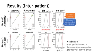
• Dataset 1: microarray (9934 genes, 29 ASD / 29 control) [1], log2-transformed
• Dataset 2: RNA-seq (22399 genes, 82 ASD / 82 control) [2], RPKM & log2-transformed
Procedure
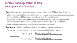
• Calculate the inter-sample and inter-gene
distance matrices for ASD/control expression
• Dissimilarity measure: 1-r (r=Pearson correlation)
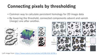
• Compute the persistent diagrams
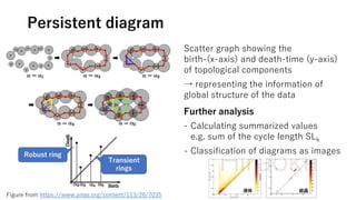
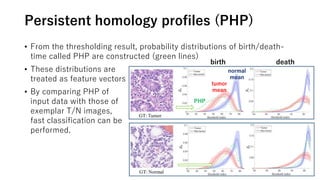
• Derive the summary values
• SDT0
= sum of death times of connected components.
• Euler characteristics = SL0 – SL1 + SL2
※SLk is sum of lifespan of connected components (k=0), rings (k=1), hollows (k=2).
[1] Voineagu et al., (2011) Nature 474, 380-384 [2] Parikshak et al., (2016) Nature 540, 423-427
Sample 1 Sample 2 Sample 3
Gene 1 0.01 0.52 …
Gene 2 0.25
Gene 3 …
Inter-sample
Inter-gene](https://image.slidesharecdn.com/200918suzuki-200918101546/85/Paper-memo-persistent-homology-on-biological-problems-7-320.jpg)
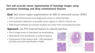
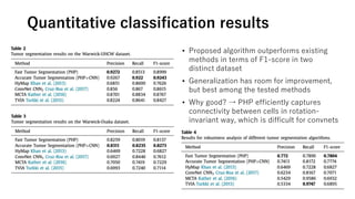
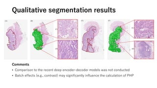

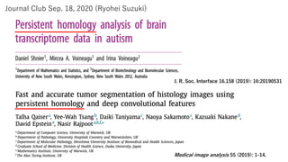
The document discusses the application of topological data analysis (TDA) in medical image analysis, specifically focusing on understanding transcriptomic characteristics in autism spectrum disorder (ASD) and colorectal cancer (CRC). It outlines the use of persistent homology to analyze high-dimensional gene expression data and proposes a CNN-based method for fast tumor-region segmentation in CRC using features derived from persistent homology. Results indicate that ASD patients exhibit more heterogeneous gene expression profiles compared to controls, and the proposed segmentation method shows improved classification performance over existing techniques.


![谷歌留痕技术 [ 𝙩𝙤𝙥 𝟮𝟯𝟯. 𝙘 𝙤𝙢 ]](https://cdn.slidesharecdn.com/ss_thumbnails/top233-260130174328-3833018c-thumbnail.jpg?width=640&height=640&fit=bounds)


