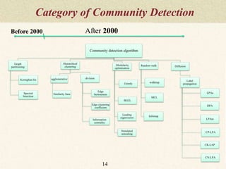
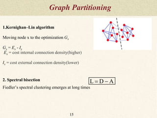
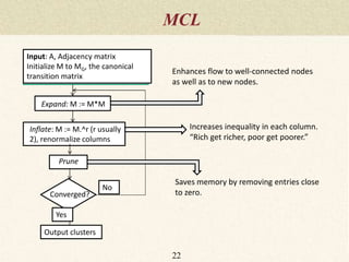
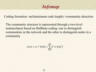
This document summarizes a thesis proposal on detecting community structure in social networks using label propagation algorithms. It begins with an introduction to complex networks and community structure detection. It then reviews several popular community detection algorithms including graph partitioning, hierarchical clustering, modularity optimization, random walks, and label propagation algorithms. The document proposes two new label propagation algorithms that incorporate measures of node and label influence to improve community detection accuracy. An example is provided to illustrate how the proposed algorithms would work.

2. Defense End
thesis issue
● Detecting Community in Social Network by Using Nodes
Labeling Diffusion
Supervisor: Dr. bouyer
Advisor: Professor Sheikholeslami
Master Reviewer : Dr. razmara
Present Student : kamal berahmand
2
Monday October, 2016th
3

3. Agenda
● Complex network
● Property of complex network
● Community structure
● Application of community structure
● Related work of community structure
● My Contribution of community structure
● Experiment
● Blind spot and Future work
3

4. Type Of Complex Network
● Social network
● W.W.W
● Internet
● Protein-protein
● Brain
● Bank & swift
● Finance & Economic
● Airline
● …………
4

5. 5

6. Properties Of Complex Network
Non-trivial property in complex network
1.Clustering Coefficient
2.The Small-world Effect
3. Degree Distributions
4. Network Resilience
5.Community Structure
6
Macro
Miso

7. Clustering coefficient and Small World
● Local clustering coefficient
● Global clustering coefficient
● Small world
● Diameter (longest shortest path)
7
path-2ofnumber
path-2closedof3 number
triplet
triangle
C 


   NNL log


Ni
ic
N
C
1

8. 32
1
)(  
k
kp
Distributer degree is Power Law

9. Robust vs. Cascade failures
node of random removal is robust
a few trigger node that can have large effects over the entire networks that the
mechanism collapsing the whole system
9

10. Community Structure
10
Before After
Distribution of links among nodes is too homogeneous ,
Complex network is global sparse and local is density that O(m)=O(n)

11. Definition of Community
Community is group of nodes which connection between nodes is
significantly higher that other nodes in the graph.
11
Vi)()( VKVK out
i
in
i    )(K
Vi
out
i
Vi
VVK in
i  


12. Application of Community Detection
1.scientic approach
community detection has important significance for understanding network
topology and analyzing network function
12

13. Engineering approach
● Knowledge graph
● Structure brain
● pharmaceutical
● Recommender system
13

14. Community detection algorithm
Graph
partitioning
Kernighan-lin
Spectral
bisection
Hierarchical
clustering
agglomerative
Similarity base
division
Edge
betweeness
Edge clustering
coefficient
Information
centrality
.Modularity
optimization
Greedy
BGLL
Simulated
annealing
Leading
eigenvector
Random walk
walktrap
MCL
Infomap
Diffusion
Label
propagation
LPAa
DPA
LPAm
CP-LPA
CK-LAP
CN-LPA
14
Before 2000 After 2000
Category of Community Detection

15. Graph Partitioning
1.Kernighan–Lin algorithm
Moving node x to the optimization Gx
Gx = Ex - Ix
Ex = cost internal connection density(higher)
Ix = cost external connection density(lower)
2. Spectral bisection
Fiedler’s spectral clustering emerges at long times
15
ADL 

16. 1- Division (top-down approach)
● 1.Grivan and Newman(GN)
● 2.Edge clustering coefficient
● 3.Information centrality
16
 


Vwu uw
uw V
vBC
,
)(


    1,1min
)3(
,)3(
,


ji
ji
JI
kk
Z
C
   
 
K.1,...,K
'





GE
GEGE
E
E
C KL
K

17. 2.Hierarchy (Agglomerative)
17
Index name formulae
Salton Index
yx kk
ydajxadj
yxs



)()(
),(
Jaccard Index
)()(
)()(
),(
ydajxadj
ydajxadj
yxs



Sorensen Index
),( yxs
yx kk
yadjxadj

 )()(
Adamic-Adar
Index
    


yadjxadjz zk
yxs
 log
1
),(
Local path 32
),( AAyxs 
Katz index
 




1
,.),(
L
l
yx
L
pathByxs
simrank
Local Random
Walk
    )(. tqtqts xyyxyxxy  
Common neighbor
Random walk base
similarity
Path similarity
Merge to node base similarity (on bottom-up approach )

18. Modularity is NP-Complete
Null model Newman
Q=(fraction of edges within communities)-(expected fraction of such edges)
18
Modularity Optimization is reduction to n
n
k
BknS 0
),(
  
ij
ijij PA
m
Q
2
1
 






ij
ji
ij
m
dd
A
m
Q
22
1

19. Modularity Optimization
1.Fast-Greedy
Global
2.Louvain(BGLL)
Local
19
 






ij
wv
ji
ij cc
m
dd
A
m
Q ),(
22
1


20. Modularity optimization
● Spectral Optimization
division into 2 communities (negative and positive elements)
)
2
(
m
kk
AB
ji
ijij 
20
• Resolution limit
2
M
M C 

21. Walktrap
21
 



n
k
t
jk
t
ik
kd
PP
jisimalarity
1
2
)(
),(

22. MCL
22
Expand: M := M*M
Inflate: M := M.^r (r usually
2), renormalize columns
Converged?
Input: A, Adjacency matrix
Initialize M to MG, the canonical
transition matrix
Yes
Output clusters
No
Prune
Enhances flow to well-connected nodes
as well as to new nodes.
Increases inequality in each column.
“Rich get richer, poor get poorer.”
Saves memory by removing entries close
to zero.

23. Infomap
23
The community structure is represented through a two-level
nomenclature based on Huffman coding: one to distinguish
communities in the network and the other to distinguish nodes in a
community
𝐿 𝑚 = 𝑞 ↷ 𝐻 𝑄 +
𝑖=1
𝑚
𝑝 𝑖
↻ 𝐻(𝑝 𝑖
Coding formation mcl(minimum code length) =community detection

24. LPA
Pros-cons LPA
Algorithm LPA
1.first initializes every node with a unique label
2. at every step each node updates Its current
label to the label shared by the maximum number
of its neighbors.
After a few iteration a single label would be
trapped inside a densely connected group of
nodes during label propagating.
Two step random
24
 vNC l
l
V maxarg
1.Select node
2.Tie break strategy
different communities may be detected in
different runs over the same network
1. time complexity liner o(m) 1.non stable
2. use of local information 2. monster
community
3. free parameter( none of
predefine any parameter)
4. none of optimization

25. 25
2.DPA
1.LPAa
3.LPAm
   
SS nNin nC
)(
max
nii
nNi
iln wspmqxC
l



)(
arg
nii
nNi
iln wspmqxC
l
)1(arg
)(



nii
nNi
iln wsfmqxC
l



)(
arg 
Rule update
Rule update
Related Work LPA
  ),(,
2
1
1
Xu
n
u
ux
xv xu
xxVuuv IIAAIIAH    








26. 26
4. LPA-CNP
5.CK-LPA
6.CeLPA
Related Work LPA
)(
2 5.0)( vl
vW 
 Vvvd
vd
vW


|)(max
)(
)(3
   vWvvW 32 )(W1 
Find community kernel
u
u
u


  1

N
ku
u
 
uvv
u vusim




1
),(max(
}}},{{maxarg|{)(PreferenceNode )(1
uvsimVuV vu 
),(maxarg svPc
i
vs
W
l
v 


              21212121 ,, VNVNGEVNVNVVEVVP  

27. Social Ranking
27

28. Node Influence and label Influence
28
Divided node in complex network :1.core 2.hub 3.bridge 4. periphery
Node influence include hub and bridge can effect negative the improve LPA
Label influence include core

29. Similarity two node
29
1
2
21
(a) (b)
Vu
vu
KK
vueCo




),(sin
Cosine (1, 2) =2/3 Cosine (1, 2) =1/2
Since the diameter of a community is 2 or 3 in complex network, the semi local
measures is an efficient alternative for computing label influence

30. Algorithm one
30
),(),(
),(),(
.)|,(



ji
ji
ijji
VCoverVCover
VCoverVCover
AVVSim



 
   


uuv
vusimilarityuK
),()(
}}},{{maxarg|{)(PreferenceNode )(1
uvsimVuV vu 
Order node ascending according by k(u)
Select node
Strategy to update
Tie break strategy: a node label is chosen based on maximum node’s strength among
neighbors.

31. Example of Algorithm one
31
Iteration 1 Iteration 2 Iteration 3
No
de
Order
updatin
g
Current label New label Order
updating
Current
label
New label Updatin
g label
Current
label
New
label
1 1 1 7 1 7 7 1 7 7
2 9 9 16 9 16 16 9 16 16
3 7 7 7 7 7 7 7 7 7
4 2 2 7 2 7 7 2 7 7
5 16 16 16 16 16 16 16 16 16
6 6 6 7 6 7 7 6 7 7
7 3 3 7 3 7 7 3 7 7
8 4 4 7 4 7 7 4 7 7
9 5 5 7 5 7 7 5 7 7
10 15 15 16 15 16 16 15 16 16
11 14 14 16 14 16 16 14 16 16
12 17 17 16 17 16 16 17 16 16
13 13 13 16 13 16 16 13 16 16
14 11 11 16 11 16 16 11 16 16
15 18 18 16 18 16 16 18 16 16
16 8 8 7 8 7 7 8 7 7
17 10 10 16 10 16 16 10 16 16
18 12 12 16 12 16 16 12 16 16
8
2
1
3
6
7
5
4
18
16
17
9
15
14
13
12
10
0
11
1.5
3.89
7.05
2.84
2.80
2.80
2.87
3.92
1.82
3.53
2.37
6.30
2.76
0.9
1.43
2.0
6
2.64
1.91
0.8
6
0.78
1.02
0.9
4

32. Algorithm two
32
 
   


uuv
vusimilarityuK
),()(
}}},{{maxarg|{)(PreferenceNode )(1
uvsimVuV vu 
Order node ascending according by k(u)
Select node
Strategy to update
IAIAAAjiSKatz  13322
)(....),( 
3322
),( AAAjiS  
Tie break strategy: computes the sum of link strength for same labels among
neighbors, choose a label of neighbors that has maximum value after summation
meand
1


33. Example of Algorithm two
33
0 .5
4
1.3
2 1.8
6
1.8
9
3.
8
1.3
3
1.3
4 2.5
2.0
3 2.8
2.0
3
2.
6
1.
6
1.
9
0.
6
1.
3
1.
7
3.
9
2.0
3
0.32
ration 1 Iteration 2 Iteration 3
Nod
e Ord
er
upd
atin
g
Curre
nt
label
New
label
Order
updatin
g
Curre
nt
label
New
label
Updati
ng
label
Current
label
New
label
1 11 11 16 11 16 16 11 16 16
2 1 1 6 1 6 6 1 6 6
3 9 9 9 9 9 16 9 2 2
4 16 16 16 16 16 16 16 16 16
5 6 6 6 6 6 6 6 6 6
6 2 2 6 2 6 6 2 6 6
7
8
10
15
10
15
16
16
10
15
16
16
16
16
10
15
16
16
16
16
9 5 5 6 5 6 6 5 6 6
10 3 3 6 3 6 6 3 6 6
11 17 17 16 17 16 16 17 16 16
12 12 12 16 12 16 16 12 16 16
13 14 14 16 14 16 16 14 16 16
14 8 8 6 8 6 6 8 6 6
15 7 7 6 7 6 6 7 6 6
16 4 4 6 4 6 6 4 6 6
17 13 13 16 13 16 16 13 16 16
18 18 18 16 18 16 16 18 16 16

34. Complexity Time
34
1.The nodes are initially labeled in time O(n).
2.Calculating node and link strength similarity ,its time complexity is O(𝑛𝑘2
).
3.Ranking nodes based on node strength that has time complexity O (n) (due to
possibility of using radix and bucket sorting algorithm in a liner time).
4.The time complexity of label update according weight link neighbor is O(kn)
that is equal to O(m).
5.Finally, the time complexity of assigning the nodes with same label to its
community is O(n).
T(n)= ( O(n𝑘2
)+ O(k)+ O(2n)+ O(m))=O(m)

35. Data Set
35
Networks N K Max k Min c Max c μ
N1
N2
N3
N4
N5
N6
1000
1000
2000
2000
5000
5000
10
10
15
15
20
20
50
50
50
50
50
50
10
20
10
20
10
20
50
100
50
100
50
100
0.1-0.8
0.1-0.8
0.1-0.8
0.1-0.8
0.1-0.8
0.1-0.8
Paramete
r name
description
N number of nodes
K average degree
Max(k) The maximum degree
𝛾 The exponent for the degree
distribution
𝛽 The exponent for community size
distribution
Min(c) The minimum community size
Max(c) The maximum community size
µ mixing parameter
Network ID Network name N E K
E1 Karate Club of Zachary 34 78 2
E2 Dolphins 62 159 2
E3 College Football 115 613 12
E4 Political Books network 105 441 3
E5 Jazz 198 2742 -----
E6 C.Elegans 453 2032 -----
E7 Email 1133 5451 -----
E8 Netscience 1589 2742 -----
E9 PowerGrid 4941 6494 -----
1.Real dataset
2.LFR Data set

36. Evaluation Criteria
2.validation data set LFR
1.validation data set Real
 






ij
wv
ji
ij cc
m
dd
A
m
Q ),(
22
1

38
Between(0,1)
Between(0,1)
 
   BHAH
BAI
BANMI


,2
),(

37. Experiment(data set real)
37
Our algorithmLPABGLLInfomapFastmodulairtyDATA SET
NumberQNumberQNumberQNumberQNumberQ
30.3923±10.391±0.2530.38130.40130.380E1
30.5524±10.410±0.28050.41860.52740.495E2
130.58210±30.571±0.180100.604120.60060.549E3
6498.05±10.481 ±0.14140.52060.52240.501E4
40.3124±10.291±0.23050.44180.28050.438E5
140.4735±10.215±.159100.440400.415140.408E6
390.54212±50.500±0.200130.541660.521170.489E7
3340.933454±60.901±0.2104060.9594420.9014030.955E8
7690.823488±50.800±.1000400.9364900.816400.934E9
Result of modularity in the algorithm one
Result of modularity in the algorithm two
LP-LPALPADPAInfomapCNMData sets
NumberQNumberQNumberQNumberQNumberQ
30.4003±10.391±0.2550.39030.40130.380E1
30.5324±10.410±0.28050.49560.52740.495E2
130.48210±30.571±0.180110.604120.60060.549E3
30.5485±10.481 ±0.14150.51060.52240.501E4
190.54212±50.500±0.200410.511660.521170.489E5
2960.933454±60.901±0.2104810.8954420.9014030.955E6
357
121
0.823
0.829
488±5
925±25
0.800±0.100
0.739± 0.141
1143
1702
0.656
0.763
490
1070
0.816
0.800
40
190
0.934
0.852
E7
E8

38. Experiment data set LFR algorithm one
38
0
0.1
0.2
0.3
0.4
0.5
0.6
0.7
0.8
0.9
1
0.1 0.2 0.3 0.4 0.5 0.6 0.7 0.8 0.9
NMI
Mixing parameter
LFR N1
0
0.1
0.2
0.3
0.4
0.5
0.6
0.7
0.8
0.9
1
0.1 0.2 0.3 0.4 0.5 0.6 0.7 0.8 0.9
NMI
Mixing parameter
LFR N2
0
0.1
0.2
0.3
0.4
0.5
0.6
0.7
0.8
0.9
1
0.1 0.2 0.3 0.4 0.5 0.6 0.7 0.8 0.9
NMI
Mixing parameter
LFR N3
0
0.1
0.2
0.3
0.4
0.5
0.6
0.7
0.8
0.9
1
0.1 0.2 0.3 0.4 0.5 0.6 0.7 0.8 0.9
NMI
Mixing parameter
LFR N4

39. Experiment data set LFR algorithm two
39
0
0.1
0.2
0.3
0.4
0.5
0.6
0.7
0.8
0.9
1
0.1 0.2 0.3 0.4 0.5 0.6 0.7 0.8 0.9
NMI
Mixing parameter
CNM
Infomap
DPA
LPA
LP-LPA
LFR N1
0
0.1
0.2
0.3
0.4
0.5
0.6
0.7
0.8
0.9
1
0.1 0.2 0.3 0.4 0.5 0.6 0.7 0.8 0.9
NMI
Mixing parameter
CNM
Infomap
DPA
LPA
LP-LPA
LFR N2
0
0.1
0.2
0.3
0.4
0.5
0.6
0.7
0.8
0.9
1
0.1 0.2 0.3 0.4 0.5 0.6 0.7 0.8 0.9
NMI
Mixing parameter
CNM
Infomap
DPA
LPA
LP-LPA
LFR N3
0
0.1
0.2
0.3
0.4
0.5
0.6
0.7
0.8
0.9
1
0.1 0.2 0.3 0.4 0.5 0.6 0.7 0.8 0.9
NMI
Mixing parameter
CNM
Infomap
DPA
LPA
LP-LPA
LFR N4

40. Blind spot and future work
● The algorithms cant detection overlapping and hiericharicty
● Experiment must be used the RC(Relaxed caveman) that it is a artificial data
set new.
● Community algorithms new have focused on multidimensional
● How to use the LPA drawback that formatting monster community to identify
node influence?
42

41. Thank you for your attention