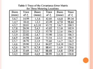
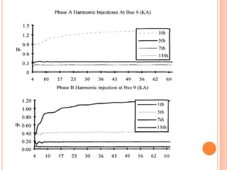
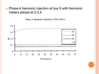
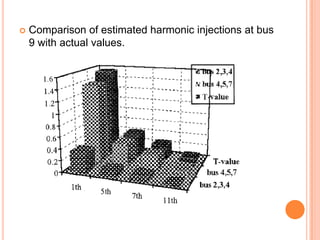
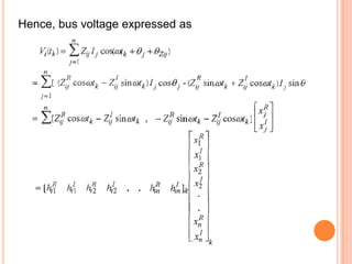
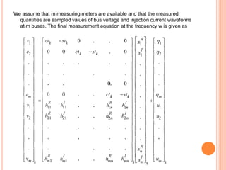
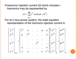
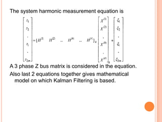
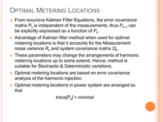
This document presents a method for using a Kalman filter to optimally locate a limited number of harmonic meters and dynamically estimate harmonic injections in an unbalanced power system. The Kalman filter formulation models harmonic injections as states and bus voltages as measurements. It determines optimal meter placements to minimize estimation error based on measurement and system noise. In a test case, the Kalman filter accurately estimated the harmonic injection at bus 9 was the major source when meters were placed at the suggested optimal locations of buses 4, 5, and 7.

1. Identification & Tracking of Harmonic Sources in a Power System using a Kalman FilterOptimal Control Theory II (ECGR 6116)Prof. Dr. KakadNikhil Kulkarni (Student ID 800696839)Adly A. Girgis, Fellow, IEEEDept. of Elect & CompEngg.Clemson UniversityClemson, SC 29634Haili Ma, Student Member, IEEEIllinois Institute of TechnologyChicago, IL 60616

2. IntroductionObjective is to solve following 2 problems using Kalman Filtering approach. 1) Optimal locations of a limited number of harmonic meters.2) Optimal dynamic estimates of harmonic source locations and their injections in unbalanced three-phase power systems. System error covariance analysis by the Kalman Filter associated with the harmonic injection estimate determines the optimal arrangement of limited harmonic meters. Based on optimally arranged harmonic metering locations, the Kalman filter then yields the optimal dyanamic estimates of harmonic injections with few noisy harmonic measurements. Harmonic injectionIts due to increasing application of non linear loads.Causes serious problems such as voltage distortion, increased losses and heating, and wrong operation of protective equipment.Due to cost, the number of harmonic meters in power systems is very limited as compare to frequency measurementHarmonic State EstimationLimitations in number of meters makes harmonic state estimations an underdetermined estimation problem.The quality of estimations is a function of the number & locations of the harmonic measurements.Non linear load devices may be 3 phase unbalanced. As a result, the unbalance of harmonic sources further complicates the harmonic sources identification problem.

3. Mathematical FormulationBus injection current expressed asc(t) = I cos(wt + θ) = I coswtcos θ- I sinwt sin θLet the state variable XR be Icos θand XI be I sin θThen 2 state variable equation for injection of current may be expressed as

4. For powers system with n buses, all bus current injections are treated as state variable,Vector W is process noise which represents the random variation of the state variable.Bus voltages are related to bus injection current by Z matrix.

5. Hence, bus voltage expressed as

6. We assume that m measuring meters are available and that the measured quantities are sampled values of bus voltage and injection current waveforms at m buses. The final measurement equation at the frequency w is given as

7. A harmonic injection current i(t) which includes rharmonics may be represented byFor an n-bus power system, the state equation representation of the harmonic injection current is

8. The system harmonic measurement equation isA 3 phase Z bus matrix is considered in the equation.Also last 2 equations together gives mathematical model on which Kalman Filtering is based.

9. A Kalman Filter AlgorithmFor simplicity mathematical model is rewritten in following formState Equation: Measurment Equation:System covariance matrices are assumed for Wkand Vk are assumed asInitial variable is assumed to be zeroInitial covariance matrix is

10. Sequential recursive computation steps for harmonic injection estimate by Kalman Filter are

11. Optimal Metering LocationsFrom recursive Kalman Filter Equations, the error covariance matrix Pk is independent of the measurements,thus Pk+1 can be explicitly expressed as a function of Pk.Advantage of Kalman filter method when used for optimal metering locations is that it accounts for the Measurement noise variance Rk and system covariance matrix Qk.These parameters may change the arrangements of harmonic metering locations up to some extend. Hence, method is suitable for Stochastic & Deterministic variations.Optimal metering locations are based on error covariance analysis of the harmonic injection.Optimal metering locations in power system are arranged so that trace[Pk] = minimal

12. Simulation TestActual power system shown in figure is use as test case

13. Power system briefCapacitors are considered as out of service.6 pulse drive is major source of harmonic.Actual 3 phase harmonic measurement data on the system is used to test the method3 phase bus voltage waveforms were observed on October 15, 1993. All signals were sampled at 7680 Hz i.e. 128 samples/cycle

14. Initial covariance estimationMeasurement error vi is unknown for specific measurement, but for stable measurement system, errors in number of measurement have certain statistical feature of normal distribution.Standard deviation of error is assumed to know.In this study, based of actual field measurement standard deviation is taken as 5%.P0(-) is denoted by σ1=3.8, σ4=1.1, σ5=3, σ6=1, σ7=2.5, σ9= 1.5.These initial parameters model the possibilities of occurrences of harmonic sources at these buses, and are determined by average load levels & prior information about harmonic sources.For buses without loads σ is chosen as 0.1Diagonal elements of Qk taken as 0.05 (p.u.)

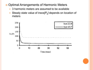
15. Optimal Arrangements of Harmonic Meters3 harmonic meters are assumed to be availableSteady state value of trace[Pk] depends on location of meters

17. Identification and Tracking of Harmonic SourcesBased on results in table I meters are placed at buses 4,5,7.Actual voltage waveform at buses 4,5,7 are sampled.No current injection were observed, i.e. load levels are low during sampling.Recursive Kalman Filter equations are used to estimate harmonic injection at all buses.Estimates of harmonic injections at all buses are very small except Bus no. 9

19. Phase A harmonic injection at bus 9 with harmonic meters placed at 2,3,4.

20. Comparison of estimated harmonic injections at bus 9 with actual values.

21. Conclusion