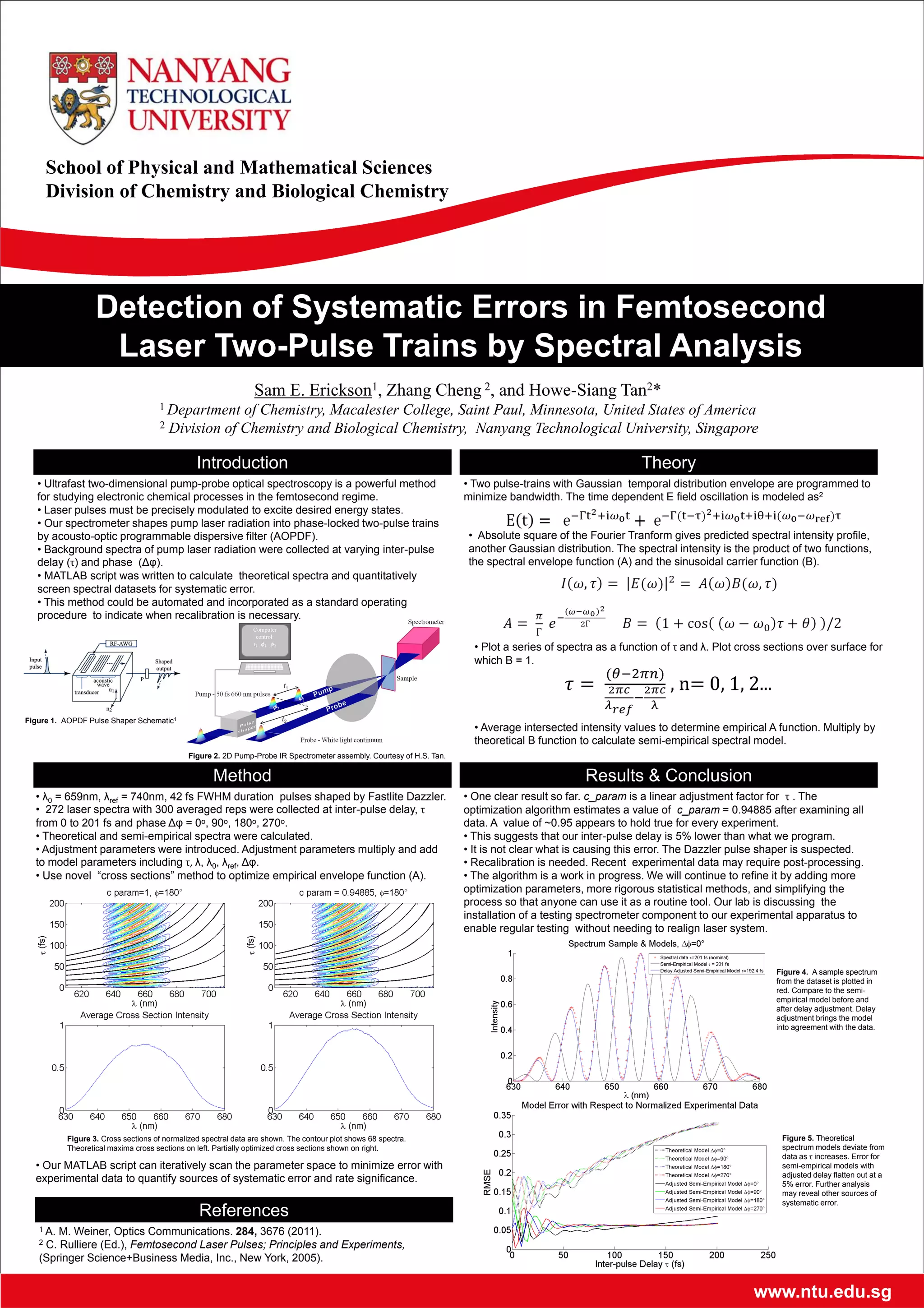
www.ntu.edu.sg
School of Physical and Mathematical Sciences
Division of Chemistry and Biological Chemistry
Introduction Theory
Method Results & Conclusion
Detection of Systematic Errors in Femtosecond
Laser Two-Pulse Trains by Spectral Analysis
Sam E. Erickson1, Zhang Cheng 2, and Howe-Siang Tan2*
1 Department of Chemistry, Macalester College, Saint Paul, Minnesota, United States of America
2 Division of Chemistry and Biological Chemistry, Nanyang Technological University, Singapore
References
• Ultrafast two-dimensional pump-probe optical spectroscopy is a powerful method
for studying electronic chemical processes in the femtosecond regime.
• Laser pulses must be precisely modulated to excite desired energy states.
• Our spectrometer shapes pump laser radiation into phase-locked two-pulse trains
by acousto-optic programmable dispersive filter (AOPDF).
• Background spectra of pump laser radiation were collected at varying inter-pulse
delay (τ) and phase (Δφ).
• MATLAB script was written to calculate theoretical spectra and quantitatively
screen spectral datasets for systematic error.
• This method could be automated and incorporated as a standard operating
procedure to indicate when recalibration is necessary.
Figure 2. 2D Pump-Probe IR Spectrometer assembly. Courtesy of H.S. Tan.
Figure 1. AOPDF Pulse Shaper Schematic1
1 A. M. Weiner, Optics Communications. 284, 3676 (2011).
2 C. Rulliere (Ed.), Femtosecond Laser Pulses; Principles and Experiments,
(Springer Science+Business Media, Inc., New York, 2005).
• Two pulse-trains with Gaussian temporal distribution envelope are programmed to
minimize bandwidth. The time dependent E field oscillation is modeled as2
• Absolute square of the Fourier Tranform gives predicted spectral intensity profile,
another Gaussian distribution. The spectral intensity is the product of two functions,
the spectral envelope function (A) and the sinusoidal carrier function (B).
• Plot a series of spectra as a function of τ and λ. Plot cross sections over surface for
which B = 1.
• Average intersected intensity values to determine empirical A function. Multiply by
theoretical B function to calculate semi-empirical spectral model.
• λ0 = 659nm, λref = 740nm, 42 fs FWHM duration pulses shaped by Fastlite Dazzler.
• 272 laser spectra with 300 averaged reps were collected at inter-pulse delay, τ
from 0 to 201 fs and phase Δφ = 0ᵒ, 90ᵒ, 180ᵒ, 270ᵒ.
• Theoretical and semi-empirical spectra were calculated.
• Adjustment parameters were introduced. Adjustment parameters multiply and add
to model parameters including τ, λ, λ0, λref, Δφ.
• Use novel “cross sections” method to optimize empirical envelope function (A).
• Our MATLAB script can iteratively scan the parameter space to minimize error with
experimental data to quantify sources of systematic error and rate significance.
Figure 3. Cross sections of normalized spectral data are shown. The contour plot shows 68 spectra.
Theoretical maxima cross sections on left. Partially optimized cross sections shown on right.
• One clear result so far. c_param is a linear adjustment factor for τ . The
optimization algorithm estimates a value of c_param = 0.94885 after examining all
data. A value of ~0.95 appears to hold true for every experiment.
• This suggests that our inter-pulse delay is 5% lower than what we program.
• It is not clear what is causing this error. The Dazzler pulse shaper is suspected.
• Recalibration is needed. Recent experimental data may require post-processing.
• The algorithm is a work in progress. We will continue to refine it by adding more
optimization parameters, more rigorous statistical methods, and simplifying the
process so that anyone can use it as a routine tool. Our lab is discussing the
installation of a testing spectrometer component to our experimental apparatus to
enable regular testing without needing to realign laser system.
Figure 4. A sample spectrum
from the dataset is plotted in
red. Compare to the semi-
empirical model before and
after delay adjustment. Delay
adjustment brings the model
into agreement with the data.
Figure 5. Theoretical
spectrum models deviate from
data as τ increases. Error for
semi-empirical models with
adjusted delay flatten out at a
5% error. Further analysis
may reveal other sources of
systematic error.

Erickson_FYP_Poster

  • 1.
    www.ntu.edu.sg School of Physicaland Mathematical Sciences Division of Chemistry and Biological Chemistry Introduction Theory Method Results & Conclusion Detection of Systematic Errors in Femtosecond Laser Two-Pulse Trains by Spectral Analysis Sam E. Erickson1, Zhang Cheng 2, and Howe-Siang Tan2* 1 Department of Chemistry, Macalester College, Saint Paul, Minnesota, United States of America 2 Division of Chemistry and Biological Chemistry, Nanyang Technological University, Singapore References • Ultrafast two-dimensional pump-probe optical spectroscopy is a powerful method for studying electronic chemical processes in the femtosecond regime. • Laser pulses must be precisely modulated to excite desired energy states. • Our spectrometer shapes pump laser radiation into phase-locked two-pulse trains by acousto-optic programmable dispersive filter (AOPDF). • Background spectra of pump laser radiation were collected at varying inter-pulse delay (τ) and phase (Δφ). • MATLAB script was written to calculate theoretical spectra and quantitatively screen spectral datasets for systematic error. • This method could be automated and incorporated as a standard operating procedure to indicate when recalibration is necessary. Figure 2. 2D Pump-Probe IR Spectrometer assembly. Courtesy of H.S. Tan. Figure 1. AOPDF Pulse Shaper Schematic1 1 A. M. Weiner, Optics Communications. 284, 3676 (2011). 2 C. Rulliere (Ed.), Femtosecond Laser Pulses; Principles and Experiments, (Springer Science+Business Media, Inc., New York, 2005). • Two pulse-trains with Gaussian temporal distribution envelope are programmed to minimize bandwidth. The time dependent E field oscillation is modeled as2 • Absolute square of the Fourier Tranform gives predicted spectral intensity profile, another Gaussian distribution. The spectral intensity is the product of two functions, the spectral envelope function (A) and the sinusoidal carrier function (B). • Plot a series of spectra as a function of τ and λ. Plot cross sections over surface for which B = 1. • Average intersected intensity values to determine empirical A function. Multiply by theoretical B function to calculate semi-empirical spectral model. • λ0 = 659nm, λref = 740nm, 42 fs FWHM duration pulses shaped by Fastlite Dazzler. • 272 laser spectra with 300 averaged reps were collected at inter-pulse delay, τ from 0 to 201 fs and phase Δφ = 0ᵒ, 90ᵒ, 180ᵒ, 270ᵒ. • Theoretical and semi-empirical spectra were calculated. • Adjustment parameters were introduced. Adjustment parameters multiply and add to model parameters including τ, λ, λ0, λref, Δφ. • Use novel “cross sections” method to optimize empirical envelope function (A). • Our MATLAB script can iteratively scan the parameter space to minimize error with experimental data to quantify sources of systematic error and rate significance. Figure 3. Cross sections of normalized spectral data are shown. The contour plot shows 68 spectra. Theoretical maxima cross sections on left. Partially optimized cross sections shown on right. • One clear result so far. c_param is a linear adjustment factor for τ . The optimization algorithm estimates a value of c_param = 0.94885 after examining all data. A value of ~0.95 appears to hold true for every experiment. • This suggests that our inter-pulse delay is 5% lower than what we program. • It is not clear what is causing this error. The Dazzler pulse shaper is suspected. • Recalibration is needed. Recent experimental data may require post-processing. • The algorithm is a work in progress. We will continue to refine it by adding more optimization parameters, more rigorous statistical methods, and simplifying the process so that anyone can use it as a routine tool. Our lab is discussing the installation of a testing spectrometer component to our experimental apparatus to enable regular testing without needing to realign laser system. Figure 4. A sample spectrum from the dataset is plotted in red. Compare to the semi- empirical model before and after delay adjustment. Delay adjustment brings the model into agreement with the data. Figure 5. Theoretical spectrum models deviate from data as τ increases. Error for semi-empirical models with adjusted delay flatten out at a 5% error. Further analysis may reveal other sources of systematic error.