Differential equation fault location algorithm with harmonic effects in power system

TELKOMNIKA Telecommunication Computing Electronics and Control
Vol. 21, No. 3, June 2023, pp. 684~694
ISSN: 1693-6930, DOI: 10.12928/TELKOMNIKA.v21i3.22503  684
Journal homepage: http://telkomnika.uad.ac.id
Differential equation fault location algorithm with harmonic
effects in power system
Izatti Md. Amin1
, Mohd Rafi Adzman1
, Haziah Abdul Hamid1
, Muhd Hafizi Idris1
,
Melaty Amirruddin1
, Omar Aliman2
1
Faculty of Electrical Engineering and Technology, Universiti Malaysia Perlis, Perlis, Malaysia
2
Faculty of Electrical and Electronic, Universiti Malaysia Pahang, Pekan, Pahang, Malaysia
Article Info ABSTRACT
Article history:
Received Dec 17, 2021
Revised Jul 12, 2022
Accepted Oct 26, 2022
About 80% of faults in the power system distribution are earth faults.
Studies to find effective methods to identify and locate faults in distribution
networks are still relevant, in addition to the presence of harmonic signals
that distort waves and create deviations in the power system that can cause
many problems to the protection relay. This study focuses on a single
line-to-ground (SLG) fault location algorithm in a power system distribution
network based on fundamental frequency measured using the differential
equation method. The developed algorithm considers the presence of
harmonics components in the simulation network. In this study, several
filters were tested to obtain the lowest fault location error to reduce the
effect of harmonic components on the developed fault location algorithm.
The network model is simulated using the alternate transients program
(ATP)Draw simulation program. Several fault scenarios have been
implemented during the simulation, such as fault resistance, fault distance,
and fault inception angle. The final results show that the proposed algorithm
can estimate the fault distance successfully with an acceptable fault location
error. Based on the simulation results, the differential equation continuous
wavelet technique (CWT) filter-based algorithm produced an accurate fault
location result with a mean average error (MAE) of less than 5%.
Keywords:
ATPDraw
CWT
Differential equation
Signal processing
Single line ground
This is an open access article under the CC BY-SA license.
Corresponding Author:
Izatti Md. Amin
Faculty of Electrical Engineering and Technology, Universiti Malaysia Perlis
02600, Arau, Perlis, Malaysia
Email: zatyamin@gmail.com
1. INTRODUCTION
Due to the problems that remain in locating the exact fault location in the distribution power
network, the utility engineers and researchers have to keep on developing new fault location algorithms to
solve this issue. After the fault, accurate location information helps the utility expertise accelerate the
network’s restoration and reconfiguration, reducing outage time and operating costs [1]-[3]. Because of that,
more efficient methods are required for better supply restoration and high-performance customer service.
In the last decades, the fault location was done naturally, such as night patrolling, visual inspection, and calls
from witnesses or customers of damages to power lines [4]. However, this primitive way does not give a
satisfying result on fault location. Thus, the substation has installed a fault indicator to record the important
information. According to [5]-[6], for determining the fault location in a distribution network, the technique
has been classified into three types; impedance-based measurement, high-frequency components of current
and voltages technique, and knowledgeable-based approaches.

TELKOMNIKA Telecommun Comput El Control 
Differential equation fault location algorithm with harmonic effects in power system (Izatti Md. Amin)
685
Nowadays, one of the main concerns for power system engineers is the presence of harmonic signals
that distort energy in the power industry [7], [8]. Nonlinear loads used by the consumer mainly cause
harmonic distortion, such as industrial using large motor speed control appliances, arc devices like the
welder, and static power converters in manufacturers of paper, textiles, steel, and others [9]. The results of
nonlinear loads caused the non-sinusoidal waveforms in the voltage and current of the power system. Thus,
the higher harmonics captured by digital fault recorders (DFR) or digital protective relays (DPRs) will affect
fault location estimation [10].
In the literature, several techniques can treat the harmonic signal. The traditional mathematical tools,
such as the standard fast Fourier transform (FFT), is a theoretical method that quickly transforms the
frequency domain signals from discrete time-domain signals. Apart from that, the FFT can be the correct
analysis tool if the signal is linear and stationary. However, directly applying the FFT algorithm may produce
inaccurate results because of spectral leakage and picket-fence effects. Short-term Fourier transform can
solve this problem by using window functions, but the flexibility of harmonic detection is reduced [11].
The wavelet transform (WT) has been used progressively for several issues in power systems analysis
involving harmonic signals. The WT does not take the fixed sinusoidal wave basis as the transform basis of
the signal compared to FFT analysis. Significantly, researchers widely use WT in signal processing to
analyze non-stationary signals [12], [13]. Identically, the average signal transform in the signal window was
in the form of the time spectrum of the whole signal in the time domain by adding small windows to the
signal waves in the time domain. In Sheng and Rovnyak [14], the modal parameters of power systems were
to analyze the origin of the small-signal oscillations and detect damping and frequency of critical modes.
The continuous wavelet technique (CWT) filter has been suggested in this research as a solution to
the harmonic appearance of fault signals. It can extract the complete time frequency of the fault signal, which
is then used in the fault algorithm to find the fault location. The faulty line with harmonic presence was also
tested with infinite impulse response (IIR) and finite impulse response (FIR) filters (FFT analysis) and
discrete wavelet technique (DWT) filters (WT analysis) as a comparison for the proposed method.
The comparison uses different signal processing with a filtered frequency range close to 50 Hz. These filters
were chosen as signal processing tools because this method is primarily used among researchers and is suitable
for a wide range of frequencies [15]-[17]. Comparative harmonic filters and their influence on estimating the
location of faults have been further addressed in sections 3 and 5. The filtered signal will then be measured
using a differential equation impedance-based technique [18]. This method was chosen because it is
appropriate for analyzing the type of earth fault signal that uses low sampling. The measured fault signal is
assumed to be received via a fault recorder or intelligent electronics devices (IED). Because it requires less
equipment, this approach is affordable and simple. Numerous characteristics, including fault resistance,
various beginning angles, and varying loads, are included in the simulation.
2. PROPOSED METHOD
The flow research design of the proposed fault location algorithm is given in Figure 1. From the circuit
model of the power system network, assume that a single line to ground fault at one of the feeders has been
detected. Three-phase voltage and current signals will be collected and sampled in the distribution substation.
Figure 1. The flow of research design

 ISSN: 1693-6930
TELKOMNIKA Telecommun Comput El Control, Vol. 21, No. 3, June 2023: 684-694
686
The recorded signals were extracted and analyzed in a Matlab environment for further analysis.
The recorded three-phase voltage and current signals comprise fundamental frequency and harmonic
components. Then, signal processing is made using filtering techniques, as described in section 3.2. Once the
harmonic has been reduced, the filtered faults voltage and current signals are used for fault location
estimation based on the differential equation method. The method of the fault distance estimation algorithm
is discussed in section 4.
3. MODELING AND SIMULATION OF POWER DISTRIBUTION NETWORK
The network was modeled and simulated by using an ATPDraw, and the result was filtered using
Matlab. This section discussed the parameters of power distribution network modeling and several types of
harmonic filters in the following subsections. After that, the filtered result will use in the next section.
3.1. Power distribution modeling
The network was modeled in ATPDraw software, and the fault location was tested at a 33 kV
distribution network with the same cable parameter. Figure 2 shows a simplified power network model
constructed using ATPDraw. This power network consists of a source, transformer, transmission line, feeder,
and harmonic load [19]-[21].
Figure 2. Simplified power distribution network model in ATPDraw
3.2. Harmonic filter
The harmonic filtering is applied to obtain the generated fault signal with the fundamental frequency
to eliminate the harmonic effect. The captured fault signals from the ATPDraw simulation were recorded and
tested with IIR, FIR, DWT, and CWT. The following sub-section discusses this work’s filtering techniques
and processes.
a) IIR filter
An IIR filter’s impulse response has an indefinite duration. An IIR digital filter’s general equation is:
𝑦(𝑛) = −Σ𝑎𝑘𝑦(𝑛 − 𝑘) + Σ𝑏𝑘𝑥(𝑛 − 𝑘) (1)
IIR filters compare fewer numbers than FIR filters, and because of that, IIR filters are excellent for high-speed
designs. The frequency response of an IIR filter can also be configured to be a discrete version of the
frequency response of an analog filter. However, IIR filters do not have a linear phase and might be unstable
if not built properly. IIR filters are also particularly susceptible to filter coefficient quantization errors
because a finite number of bits represents the filter coefficient [22]. The IIR Notch single filter has been used
for filtering the 50 Hz signal.
b) FIR filter
A FIR digital filter is one whose impulse response is of limited duration. The general difference
equation for an FIR digital filter is:
𝑦(𝑛) = Σ𝑏𝑘𝑥(𝑛 − 𝑘) (2)
The essence of the FIR filter is to weigh and sum the values of the past time. Compared to the IIR filter, there is
no need to feedback on the output, so the structure is simple and easy to implement in programming [23].
The FIR lowpass filter signals below 50 Hz and FIR bandpass in the 50-51Hz range were used in this research.

687
c) DWT
The DWT is a multi-resolution wavelet analysis where the signal analysis decomposes in multiple
bands [24]. The DWT provides each frequency in octave scale and two spatial-temporal arrangements in the
analyzed signal to solve and treat more advanced problems. However, the disadvantage is that it depends on
the total energy of the moving wavelet signals on several scales in signal shifting downwards [25]. This
technique employs two sets of functions, called scaling function ∅ and wavelet function 𝜑. The mathematical
expression for DWT is given by [26].
𝐷𝑊𝑇(𝑚, 𝑛) =
1
√2𝑚
∑ 𝑓(𝑘)𝜑 (
𝑛−𝑘2𝑚
2𝑚 )
𝑘 (3)
The recorded signals were filtered in a series of two type types of digital filtering techniques: the high pass filter
and the low pass filter. Thus, the signal is decomposed into component approximation (A) and detail (D)
coefficients [25]. The decomposition process can be iterated, called the wavelet decomposition tree, as shown in
Figure 3. Figure 3 shows four levels of DWT filter were used by filtering the signal between 0 and 62.5 Hz with
Daubechies 4 of the family type of DWT in this research.
Figure 3. Wavelet decomposition tree
d) CWT
The CWT is useful for assessing non-stationary objects’ dynamic features. The CWT is also an
excellent tool for determining whether or not a symptom is stationary in the global sense. In a non-stationary
signal, CWT is utilized to identify stationary data signals [25]. The wavelet generally is a complex value
function that is accurate for only one or a few cycles of the oscillating waveform. Wavelet is used in an
integral transform as a kernel function. The signal 𝑠(𝑡) shows as [27]-[29].
C(a, b) = ∫ s(t). ψ
̅a.b(t)dt
+∞
-∞
(4)
The (5) represents CWT, where a and b are continuous parameters [29]. Wavelets with different ‘𝑎’, ‘𝑏’
parameters create a family with an essential mother wavelet function 𝛹(𝑡).
𝜓𝑎,𝑏(𝑡) =
1
√𝛪𝑎𝛪
𝜓 (
𝑡−𝑏
𝑎
) 𝑑𝑡 (5)
The mother wavelet 𝛹(𝑡) must be short and oscillatory, and it must have zero average and effectively limited
duration. The (4) has the location ‘b’ as a position scale and duration scale (duration shifting factor) as the
scale ‘𝑎’. The 𝛹 in (5) is known as the complex conjugate of 𝛹, and the output of CWT would be the
wavelet coefficient denoted as 𝐶(𝑎, 𝑏). CWT is used to extract the 50 Hz filtered signal.
4. FAULT LOCATION ALGORITHM
The filtered voltage and current signal are used in the fault location algorithm to estimate the
distance of the fault location. In a single-phase-to-ground fault, the fault loop represents by a series of
connections of the line’s symmetrical component impedances [19]. The fault inductance of a faulty line is
composed of positive, negative, and zero sequences in series connection as [29], [30].

 ISSN: 1693-6930
688
𝐿𝑓 =
1
3
(𝐿𝑡,𝑝 + 𝐿𝑡,𝑛 + 𝐿𝑡,𝑜) . 𝑙 (6)
The differential equation method is chosen to estimate the fault location in this study. The impedance
measurement from a different algorithm is developed from a simple model of the fault loop, the faulted line
from a typical 𝑅-𝐿 circuits series. The current and voltage samples extracted, for example, recorded from
digital fault recorder (DFR) installed in the power system substation, can be applied to this model for a
calculated parameter. The differential equation from a basic equation form as in (7).
𝑢(𝑡) = 𝑅𝑖(𝑡) + 𝐿
𝑑𝑖(𝑡)
𝑑𝑡
(7)
From voltage and current samples, the unknown 𝑅 and 𝐿 were solved by using the following:
𝑅 = [
(𝑣𝑘+1+𝑣𝑘)(𝑖𝑘+2−𝑖𝑘+1)−(𝑣𝑘+2+𝑣𝑘+1)(𝑖𝑘+1−𝑖𝑘)
(𝑖𝑘+1+𝑖𝑘)(𝑖𝑘+2−𝑖𝑘+1)−(𝑖𝑘+2+𝑖𝑘+1)(𝑖𝑘+1−𝑖𝑘)
] (8)
𝐿 =
∆𝑡
2
[
(𝑖𝑘+1+𝑖𝑘)(𝑣𝑘+2+𝑣𝑘+1)−(𝑖𝑘+2+𝑖𝑘+1)(𝑣𝑘+1+𝑣𝑘)
(𝑖𝑘+1+𝑖𝑘)(𝑖𝑘+2−𝑖𝑘+1)−(𝑖𝑘+2+𝑖𝑘+1)(𝑖𝑘+1−𝑖𝑘)
] (9)
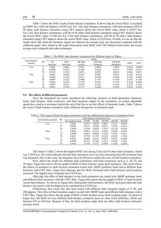
In this work, only the inductance given in (6) and (9) was used to estimate the fault distance. The mean
average error (MAE) equation calculates the fault estimation error. Based on the result, the lowest MAE
represents a good result. It shows that the estimated fault location is near the exact fault location.
5. RESULTS AND DISCUSSION
This section discusses the result of using the differential equation-based fault location technique
described in the previous section. Figure 4 shows an example of the harmonic and without harmonic current
signal captured during the simulation. A nonlinear load causes the harmonic at the end of this system.
(a) (b)
Figure 4. The current signal: (a) without harmonic and (b) with harmonic having nonlinear loads
As shown in Figure 4(a), the current signal shows a pure sine waveform. In contrast, in Figure 4(b),
the harmonic current signal shows a distorted waveform and produces a non-sinusoidal waveform.
The waveform will be filtered with several filter types to eliminate the harmonic current for accurate fault
location estimation. The result will be discussed in the following subsection.
5.1. The effect of harmonic filter
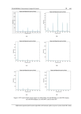
Figure 5(a) illustrates the FFT of a harmonically generated fault signal current. The fault distance is 5 km
with 100 HP of nonlinear loads. The present signal was then filtered with a different type of filter. The figure also
represents the FFT of filtered results obtained using several types of filters, including IIR (Figure 5(b)), lowpass
FIR (Figure 5(c)), bandpass FIR (Figure 5(d)), DWT (Figure 5(e)), and CWT (Figure 5(f)). Figure 5(a) indicates
the outcome of the current signal with the third, fifth, seventh, and ninth harmonic components. The result
demonstrates that the harmonic component was successfully filtered out using FIR in Figure 5(d), and CWT in
Figure 5(f). In contrast, the IIR filter in Figure 5 (b) shows a worse result than other filtering techniques.
(f ile simplenew.pl4; x-v ar t) c:XA -BA
0.16 0.18 0.20 0.22 0.24 0.26 0.28 0.30 0.32
[s]
-40
-30
-20
-10
0
10
20
30
40
[mA]
(f ile simplenew.pl4; x-v ar t) c:XA -BA
0.18 0.20 0.22 0.24 0.26 0.28 0.30 0.32
[s]
-1.5
-1.0
-0.5
0.0
0.5
1.0
1.5
[A]

689
(a) (b)
(c) (d)
(e) (f)
Figure 5. FFT result of fault current signal: (a) without filter, (b) with IIR filter, (c) with FIR lowpass,
(d) with FIR bandpass, (e) with DWT, and (f) with CWT

 ISSN: 1693-6930
690
Table 1 shows the MAE result of fault distance estimation. It shows that the lowest MAE is recorded
as 0.0061 km, while the highest is 0.5503 km. For 1 km fault distance estimations, with fault resistance (Rf) of
50 ohms, fault distance estimation using CWT analysis shows the lowest MAE value, which is 0.0471 km.
For 3 km fault distance estimations, with Rf of 50 ohms, fault distance estimation using CWT analysis shows
the lowest MAE value, 0.1348 km. For 5 km fault distance estimations, with Rf of 50 ohms, fault distance
estimation using CWT analysis shows the lowest MAE value, which is 0.2254 km. Overall, we can see that the
results show that when the harmonic signal was filtered, the average error was decreased compared with the
unfiltered signal. Also, based on the result observation, most MAE with CWT-filtered result shows the lowest
average error compared with other techniques.
Table 1. The MAE fault distance estimation for different types of filters
Fault distance
(actual)
Rf
MAE.
No
harmonic
With
harmonic
IIR filter
(notch)
FIR filter
(lowpass)
FIR filter
(bandpass)
DWT CWT
1 km 0 0.0001 0.0061 0.5437 0.0036 0.0042 0.0636 0.0050
25 0.0008 0.0531 0.3588 0.0238 0.0312 0.0652 0.0227
50 0.0210 0.7823 0.4931 0.0505 0.0632 0.0841 0.0471
3 km 0 0.0001 0.0205 0.5617 0.0093 0.0312 0.1892 0.0142
25 0.0004 0.1670 0.4177 0.0748 0.0978 0.1961 0.0648
50 0.0007 0.3222 0.5988 0.1547 0.1939 0.2533 0.1348
5 km 0 0.0002 0.0378 0.5760 0.0143 0.1793 0.3186 0.0209
25 0.0007 0.2911 0.4753 0.1301 0.1703 0.3278 0.1105
50 0.0012 0.5503 0.7577 0.2634 0.3303 0.4235 0.2254
5.2. The effects of different parameter
Next, the simulation test result considered the following variation of fault parameters: harmonic
loads, fault distance, fault resistances, and fault inception angles. In the simulation, six pulses adjustable
speed drive used as a nonlinear load at the end of the line to see the effects of harmonic loads. Table 2 shows
the result of fault location estimation with a different horsepower of nonlinear loads.
Table 2. The result of fault location estimation with the different horsepower of nonlinear loads
Fault distance (actual) RF
Fault distance (estimation, km)
No nonlinear load 25 HP 50 HP 100 HP 200 HP 500 HP
1 km 0 0.0001 0.0015 0.0030 0.0061 0.0122 0.0289
25 0.0008 0.0131 0.0264 0.0531 0.1078 0.2612
50 0.0010 0.0259 0.0520 0.7823 0.2138 0.4146
3 km 0 0.0001 0.0051 0.0102 0.0205 0.0409 0.6595
25 0.0008 0.0413 0.0829 0.1670 0.3395 0.8327
50 0.0017 0.0795 0.1597 0.3222 0.6595 1.3303
5 km 0 0.0001 0.0095 0.0189 0.0378 0.0755 0.1694
25 0.0008 0.0719 0.1444 0.2911 0.5929 1.4743
50 0.0016 0.1356 0.2725 0.5503 1.1296 2.2858
The result in Table 2 shows the highest MAE was during 5 km and 50 ohms fault resistance, which
was 2.2858 km. The result indicates that the fault estimation error was also increased when the nonlinear load
was increased. Due to this issue, the harmonic must be filtered to reduce the error of fault location estimation.
Next, shows the results for different fault estimations with fault resistances such as 5, 10, 25, and
50 ohms. Figure 6(a) shows the bar graph of MAE of fault location versus fault resistance. This result shows
the effects of resistance to fault location estimation tested with 100HP nonlinear loads and at different fault
locations with CWT filter. Figure 6(a) indicates that the MAE increased when fault distance and resistance
increased. The highest error estimated was 0.2254 km.
After that, the effect of fault distance on the fault estimation was tested with 100HP nonlinear loads
and different fault resistance with the CWT filter. Figure 6(b) shows the bar graph of MAE of fault location
versus fault distance. As shown in Figure 6(b), during fault with harmonic, the MAE increased when the fault
distance was raised, with the highest error estimated was 0.2254 km.
Furthermore, this circuit has also been tested with different fault inception angles of 0, 90, and
180 degrees. This effect of fault inception angle is tested with 100HP loads and different fault distances with a
CWT filter. Figure 6(c) shows the bar graph of MAE of fault location versus fault inception angle. As shown in
Figure 6(c), the MAE of every different fault distance estimation does not show much difference, which was
between 0.01 to 0.03 km. Because of that, the fault inception angle does not affect fault location estimation
accuracy much.

691
(a)
(b)
(c)
Figure 6. The bar graph of MAE of fault location estimation versus: (a) fault resistance, (b) fault distance,
and (c) fault inception angle

 ISSN: 1693-6930
692
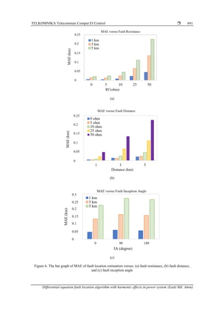
6. CONCLUSION
Overall, it can be concluded that using the differential equation CWT filter-based algorithm
produced the most accurate fault location result compared with three other filter techniques tested in this
work. The result shows that using the proposed fault location algorithm, the mean average error (MAE) gives
a result accurately with an error of less than 5%. Furthermore, suppose the fault-generated signal having a
harmonic component is used for fault location estimation. In that case, the fault distance, resistance, and
nonlinear load can significantly affect the fault location estimation.
ACKNOWLEDGEMENTS
The authors would like to acknowledge the support from the Faculty of Electrical Engineering
Technology, Universiti Malaysia Perlis (UNIMAP) for the FTKE Research Activities Fund and the support from
the Fundamental Research Grant Scheme (FRGS) under a grant number of FRGS/1/2019/TK07/UNIMAP/ 03/2
from the Ministry of Higher Education Malaysia.
REFERENCES
[1] R. Das and D. Novosel, “Review of Fault Location Techniques for Transmission and Subtransmission Lines,” in Proc. of the 54th
Annual Georgia Tech Fault and Disturbance Analysis Conference, 2000, doi: 10.13140/2.1.2143.7767.
[2] S. S. Gururajapathy, H. Mokhlis, and H. A. Illias, “Fault Location Technique in Power Distribution Systems with Distributed
Generation: A Review,” Renewable and Sustainable Energy Reviews, vol. 74, pp. 949-958, 2017, doi: 10.1016/j.rser.2017.03.021.
[3] M. Rezamand, M. Kordestani, R. Carriveau, D. S. -K. Ting, M. E. Orchard, and M. Saif, “Critical wind turbine components
prognostics: a comprehensive review,” IEEE Transactions on Instrumentation and Measurement, vol.69, no.12, pp. 9306-9328,
2020, doi: 10.1109/TIM.2020.3030165.
[4] M. M. Saha, J. Izykowski, and E. Rosolowski, Fault Location Algorithm on Power Networks, London: Springer-Verlag, 2010,
doi: 10.1007/978-1-84882-886-5.
[5] G. Buiges, V. Valverde, I. Zamora, J. Mazón, and E. Torres, “Signal Injection Techniques for Fault Location in Distribution
Networks,” 2012 International Conference on Renewable Energies and Power Quality, 2012, doi: 10.24084/REPQJ10.330.
[6] N. S. B. Jamili, M. R. Adzman, S. R. A. Rahim, S. M. Zali, M. Isa, and H. Hanafi, “Evaluation of earth fault location algorithm in
medium voltage distribution network with the correction technique,” International Journal of Electrical and Computer
Engineering, vol. 9, no. 3, pp. 1987-1996, 2019, doi: 10.11591/IJECE.V9I3.PP1987-1996.
[7] Y. Chen, J. Yin, Z. Li, and R. Wei, “Single-Line-to-Ground fault location in resonant grounded systems based on faults
distortions,” IEEE Access, vol. 9, pp. 34325-34337, 2021, doi: 10.1109/ACCESS.2021.3061211.
[8] S. Datta, A. Chattopadhyaya, S. Chattopadhyaya, and A. Das, “Harmonic distortion, inter-harmonic group magnitude and discrete
wavelet transformation based statistical parameter estimation for line to ground fault analysis in microgrid system,” Michael
Faraday IET International Summit 2020 (MFIIS 2020), 2020, pp. 177-184, doi: 10.1049/icp.2021.1087.
[9] S. A. Ali, “Modelling of power networks by ATP-Draw for harmonics propagation study,” Transactions on Electrical and
Electronics Materials, vol. 14, no. 6, pp. 283-290, 2013, doi: 10.4313/TEEM.2013.14.6.283.
[10] C. Galvez and A. Abur, “Fault location in power networks using sparse set of digital fault recorders,” IEEE Transactions on
Smart Grid, vol. 13, no. 5, pp. 3468-3480, 2022, doi: 10.1109/TSG.2022.3168904.
[11] J. Bruna and J. J. Melero, “Selection of the most suitable decomposition filter for the measurement of fluctuating harmonics,”
IEEE Transactions on Instrumentation and Measurement, vol. 65, no. 11, pp. 2587-2594, 2016, doi: 10.1109/TIM.2016.2588586.
[12] M. S. Sachdev, M. A. Baribeau, “A New Algorithm for Digital Impedance Relays,” IEEE Transactions on Power Apparatus and
Systems, vol. PAS-98, no. 6, pp. 2232-2240, 1997, doi: 10.1109/TPAS.1979.319422.
[13] M. V. Subbarao and P. Samundiswary, “Time-frequency analysis of non-stationary signals using frequency slice wavelet
transform,” 2016 10th International Conference on Intelligent Systems and Control (ISCO), 2016, pp. 1-6,
doi: 10.1109/ISCO.2016.7726999.
[14] Y. Sheng and S. M. Rovnyak, “Decision Tree-Based Methodology for High Impedance Fault Detection,” IEEE Transactions on
Power Delivery, vol. 19, no. 2, pp. 533-536, 2004, doi: 10.1109/TPWRD.2003.820418.
[15] M. Z. T. Nasrollah, E. Prasetyono, D. O. Anggiawan, “Mapping detection of series arc fault based on Fast Fourier Transform,”
2021 International Electronics Symposium (IES), 2021, pp. 582-587, doi: 10.1109/IES53407.2021.9594018.
[16] M. -F. Guo, X. -D. Zeng, D. -Y. Chen, and N. -C. Yang, “Deep learning-based earth fault detection using continuous wavelet
transform and convolutional neural network in resonant grounding distribution system,” IEEE Sensors Journal, vol. 18, no. 3,
pp. 1291-1300, 2018, doi: 10.1109/JSEN.2017.2776238.
[17] X. Tang, Z. Zhang, Q. Huang, and Y. Gong, “Fault location and fault time recognition of power system based on wavelet
transform,” in 2019 IEEE Innovative Smart Grid Technologies - Asia (ISGT Asia), 2019, pp. 689-692, doi: 10.1109/ISGT-
Asia.2019.8881101.
[18] S. El-Tawab, H. S. Mohamed, A. Refky, and A. M. A. -Aziz, “Self-healing of active distribution networks by accurate fault
detection, classification, and location,” Journal of Electrical and Computer Engineering, 2022, doi: 10.1155/2022/4593108.
[19] F. E. Perez, E. Orduña, and G. Guidi, “Adaptive wavelets applied to fault classification on transmission lines,” IET Generation
Transmission and Distribution, vol. 5, no. 7, pp. 694–702, 2011, doi: 10.1049/iet-gtd.2010.0615.
[20] J. M. -Velasco, Transient Analysis of Power Systems: A Practical Approach, John Wiley & Sons, Inc, 2019,
doi: 10.1002/9781119480549.
[21] M. Ceraolo, “MC’s PLOTXY-A general purpose plotting and post processing open-source tool,” SoftwareX, vol. 9, pp. 282-287,
2019, doi: 10.1016/j.softx.2019.01.017.
[22] L. Litwin, “FIR and IIR digital filters,” IEEE Potentials, vol. 19, no. 4, pp 28-31, 2000, doi: 10.1109/45.877863.
[23] H. Zhao, L. Zhang, J. Liu, C. Zhang, J. Cai, and L. Shen, “Design of low-order FIR filter for high-frequency-square-wave voltage
injection method of the PMLSM used in Maglev train,” Electronics, vol. 9, no. 5, 2020, doi: 10.3390/electronics9050729.

693
[24] M. I. Zaki, R. A. E. Seheimy, G. M. Amer, and F. M. A. E. Enin, “Integrated discrete wavelet transform-based faulted phase
identification for multi-terminals power systems,” in 2017 Nineteenth International Middle East Power Systems Conference
(MEPCON), 2017, pp. 503-509, doi: 10.1109/MEPCON.2017.8301227.
[25] D. Paul, S. K. Mohanty, and C. K. Panigrahi, “Classification of power swing using wavelet and convolution neural network,” in
2019 IEEE 5th International Conference for Convergence in Technology (I2CT), 2019, pp. 1-6,
doi: 10.1109/I2CT45611.2019.9033724.
[26] A. C. Adewole, R. Tzoneva, and S. Benardien, “Distribution network fault section identification and fault location using wavelet
entropy and neural network,” Applied Soft Computing, vol. 46, pp 296-306, 2016, doi: 10.1016/j.asoc.2016.05.013.
[27] M. R. Adzman, D. Topolanek, M. Lehtonen, and P. Toman, “An earth fault location scheme for isolated and compensated neutral
distribution systems,” International Review Electrical Engineering (IREE), vol. 8, no. 5, pp. 1520-1531, 2013. [Online].
Available:
https://www.researchgate.net/publication/283802417_An_Earth_Fault_Location_Scheme_for_Isolated_and_Compensated_Neutr
al_Distribution_Systems
[28] A. Belkhou, A. Achmamad, and A. Jbari, “Classification and diagnosis of myopathy EMG signals using continuous wavelet
transform,” 2019 Scientific Meeting on Electrical-Electronics & Biomedical Engineering and Computer Science (EBBT), 2019,
doi: 10.1109/EBBT.2019.8742051.
[29] Z. Radojevic, V. Terzija, G. Preston, S. Padmanabhan, and D. Novosel, “Smart Overhead Lines Autoreclosure Algorithm Based
on Detailed Fault Analysis,” IEEE Transactions on Smart Grid, vol. 4, no. 4, pp. 1829-1838, 2013,
doi: 10.1109/TSG.2013.2260184.
[30] P. S. Bhowmik, P. Purkait, and K. Bhattacharya, “A Novel wavelet transform aided neural network based transmission line fault
analysis method,” International Journal of Electrical Power & Energy Systems, vol. 31, no. 5, pp. 213-219, 2009,
doi: 10.1016/j.ijepes.2009.01.005.
BIOGRAPHIES OF AUTHORS
Izatti Md. Amin received the B.Sc. and M.Sc. degrees in electrical engineering
from Universiti Tun Hussein Onn (UTHM), Johor, Malaysia, in 2012 and 2014. She is
pursuing her Ph.D. in Electrical Engineering at Universiti Malaysia Perlis (UNIMAP), Perlis,
Malaysia. Her research interests include high voltage and signal processing applications for
power system planning, operation, and control. She can be contacted at email:
zatyamin@gmail.com.
Mohd Rafi Adzman was born in Selangor, Malaysia, in June 1976. He received
the M.Sc. degree in power systems and high voltage engineering from Helsinki University of
Technology, Finland, in 2006 and a D.Sc. degree in technology from Aalto University,
Finland, in 2014. In 2001, he was a Project Engineer with Foxboro, Malaysia. Then, he
joined Power Cable Malaysia, as an Electronics Engineer, in 2003. He has been with the
School of Electrical System Engineering, Universiti Malaysia Perlis (UniMAP), since 2004.
He has also been with University Malaysia Perlis (UniMAP), since 2006, as a Lecturer. He is
currently an associate professor at the Faculty of Electrical Engineering Technology,
UniMAP. His current research interests include renewable energy, power system distribution
automation, fault localization, power quality, and artificial intelligent application in power
systems. He is a member of the International Association of Engineers (IAENG) and the
Board of Engineers Malaysia (BEM), Malaysia. He can be contacted at email:
mohdrafi@unimap.edu.my.
Haziah Abdul Hamid received the B.Sc. and M.Sc. degrees in electrical
engineering from Universiti Teknologi Malaysia (UTM), Johor, Malaysia, in 2000 and 2002
and a D.Sc. degree in electrical engineering from Cardiff University, United Kingdom, in
2013. She is currently an associate professor at the Faculty of Electrical Engineering
Technology, Universiti Malaysia Perlis (UniMAP). Her research interests include high
voltage, grounding systems, and switching transients. She can be contacted at email:
haziah@unimap.edu.my.

 ISSN: 1693-6930
694
Muhd Hafizi Idris received the M.Sc. degree in electrical engineering from
Universiti Teknologi Malaysia (UTM), Johor, Malaysia, in 2010 and a D.Sc. degree in
electrical engineering from Universiti Malaysia Perlis (UNIMAP), Perlis, Malaysia in 2022.
He is a senior lecturer at the Faculty of Electrical Engineering Technology, UniMAP. His
research interests include high voltage, power system protection, fault localization, and
substation automation. He can be contacted at email: hafiziidris@unimap.edu.my.
Melaty Amirruddin received the B.Sc. and M.Sc. degrees in electrical
engineering from Universiti Teknologi Petronas (UTP), Perak, Malaysia, and Universiti
Teknologi Malaysia (UTM), Johor, Malaysia, in 2009 and 2011. She is currently pursuing
her Ph.D. in Electrical Engineering at Universiti Malaysia Perlis (UNIMAP), Perlis,
Malaysia. She is a lecturer at the Faculty of Electrical Engineering Technology, UniMAP.
Her research interests include high voltage and signal processing applications for power
system planning, operation, and control. She can be contacted at email:
melaty@unimap.edu.my.
Omar Aliman received B.Sc. degrees in electrical engineering and M.Sc.
degrees in optical engineering from Hanyang University, Seoul, Korea, and Universiti
Teknologi Malaysia (UTM), Johor, Malaysia, in 1997 and 2002. He is a lecturer at the
Faculty of Electrical and Electronic Engineering, UMP. His research interests include power
system analysis, distributed generation, solar energy, and arc flash analysis. He can be
contacted at email: omaraliman@ump.edu.my.

Differential equation fault location algorithm with harmonic effects in power system

More Related Content

Similar to Differential equation fault location algorithm with harmonic effects in power system

More from TELKOMNIKA JOURNAL

Recently uploaded

Differential equation fault location algorithm with harmonic effects in power system