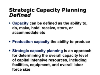
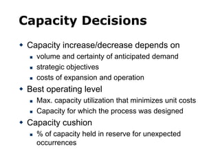
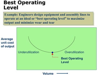
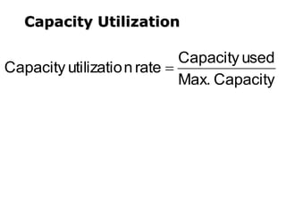
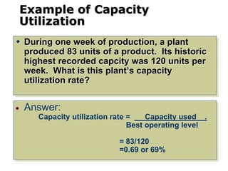
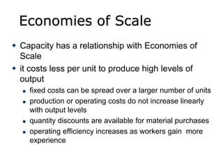
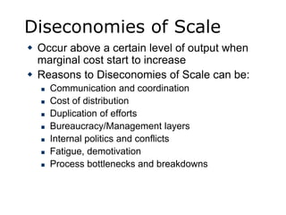
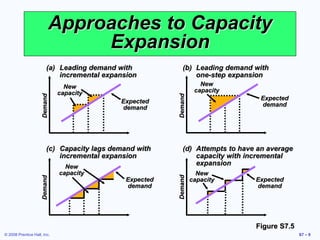
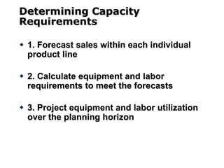
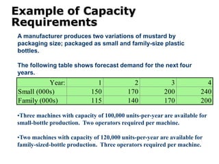
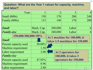
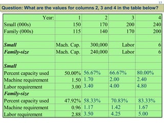
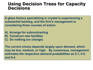
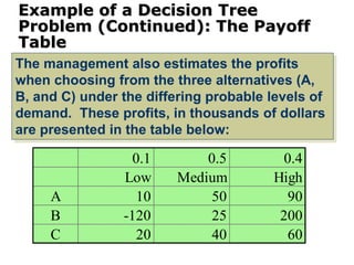
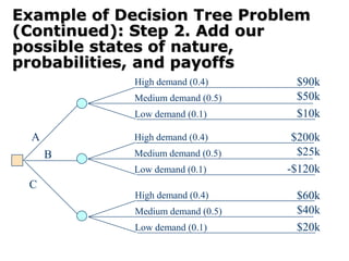
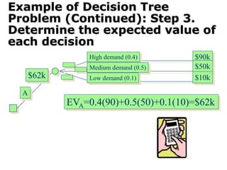
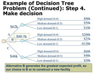
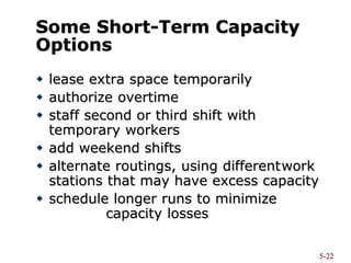
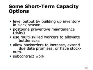
Operations Management
Instructor: Dr. Rizwan Ahmed
Capacity Management
Strategic Capacity Planning
Defined
 Capacity can be defined as the ability to,
do, make, hold, receive, store, or
accommodate etc
 Production capacity the ability to produce
 Strategic capacity planning is an approach
for determining the overall capacity level
of capital intensive resources, including
facilities, equipment, and overall labor
force size
Capacity Decisions
 Capacity increase/decrease depends on
 volume and certainty of anticipated demand
 strategic objectives
 costs of expansion and operation
 Best operating level
 Max. capacity utilization that minimizes unit costs
 Capacity for which the process was designed
 Capacity cushion
 % of capacity held in reserve for unexpected
occurrences
Best Operating
Level
Example: Engineers design equipment and assembly lines to
operate at an ideal or “best operating level” to maximize
output and minimize wear and tear
Underutilization
Best Operating
Level
Average
unit cost
of output
Volume
Overutilization
Capacity Utilization
Capacity
Max.
used
Capacity
rate
n
utilizatio
Capacity 
Example of Capacity
Utilization
 During one week of production, a plant
produced 83 units of a product. Its historic
highest recorded capcity was 120 units per
week. What is this plant’s capacity
utilization rate?
 Answer:
Capacity utilization rate = Capacity used .
Best operating level
= 83/120
=0.69 or 69%
Economies of Scale
 Capacity has a relationship with Economies of
Scale
 it costs less per unit to produce high levels of
output
 fixed costs can be spread over a larger number of units
 production or operating costs do not increase linearly
with output levels
 quantity discounts are available for material purchases
 operating efficiency increases as workers gain more
experience
Diseconomies of Scale
 Occur above a certain level of output when
marginal cost start to increase
 Reasons to Diseconomies of Scale can be:
 Communication and coordination
 Cost of distribution
 Duplication of efforts
 Bureaucracy/Management layers
 Internal politics and conflicts
 Fatigue, demotivation
 Process bottlenecks and breakdowns
© 2008 Prentice Hall, Inc. S7 – 9
Approaches to Capacity
Expansion
(a) Leading demand with
incremental expansion
Demand
Expected
demand
New
capacity
(b) Leading demand with
one-step expansion
Demand
New
capacity
Expected
demand
(d) Attempts to have an average
capacity with incremental
expansion
Demand
New
capacity Expected
demand
(c) Capacity lags demand with
incremental expansion
Demand
New
capacity
Expected
demand
Figure S7.5
Determining Capacity
Requirements
 1. Forecast sales within each individual
product line
 2. Calculate equipment and labor
requirements to meet the forecasts
 3. Project equipment and labor utilization
over the planning horizon
Example of Capacity
Requirements
A manufacturer produces two variations of mustard by
packaging size; packaged as small and family-size plastic
bottles.
The following table shows forecast demand for the next four
years.
Year: 1 2 3 4
Small (000s) 150 170 200 240
Family (000s) 115 140 170 200
•Three machines with capacity of 100,000 units-per-year are available for
small-bottle production. Two operators required per machine.
•Two machines with capacity of 120,000 units-per-year are available for
family-sized-bottle production. Three operators required per machine.
Year: 1 2 3 4
Small (000s) 150 170 200 240
Family (000s) 115 140 170 200
Small Mach. Cap. 300,000 Labor 6
Family-size Mach. Cap. 240,000 Labor 6
Small
Percent capacity used 50.00%
Machine requirement 1.50
Labor requirement 3.00
Family-size
Percent capacity used 47.92%
Machine requirement 0.96
Labor requirement 2.88
Question: What are the Year 1 values for capacity, machine,
and labor?
150,000/300,000=50%
At 2 operators for
100,000, it takes 3
operators for 150,000
At 1 machine for 100,000, it
takes 1.5 machines for 150,000
©The McGraw-Hill Companies, Inc., 2004
12
Year: 1 2 3 4
Small (000s) 150 170 200 240
Family (000s) 115 140 170 200
Small Mach. Cap. 300,000 Labor 6
Family-size Mach. Cap. 240,000 Labor 6
Small
Percent capacity used 50.00%
Machine requirement 1.50
Labor requirement 3.00
Family-size
Percent capacity used 47.92%
Machine requirement 0.96
Labor requirement 2.88
Question: What are the values for columns 2, 3 and 4 in the table below?
56.67%
1.70
3.40
58.33%
1.17
3.50
66.67%
2.00
4.00
70.83%
1.42
4.25
80.00%
2.40
4.80
83.33%
1.67
5.00
13
©The McGraw-Hill Companies, Inc., 2004
Using Decision Trees for Capacity
Decisions
A glass factory specializing in crystal is experiencing a
substantial backlog, and the firm's management is
considering three courses of action:
A) Arrange for subcontracting
B) Construct new facilities
C) Do nothing (no change)
The correct choice depends largely upon demand, which
may be low, medium, or high. By consensus, management
estimates the respective demand probabilities as 0.1, 0.5,
and 0.4.
Example of a Decision Tree
Problem (Continued): The Payoff
Table
0.1 0.5 0.4
Low Medium High
A 10 50 90
B -120 25 200
C 20 40 60
The management also estimates the profits
when choosing from the three alternatives (A,
B, and C) under the differing probable levels of
demand. These profits, in thousands of dollars
are presented in the table below:
Example of a Decision Tree
Problem (Continued): Step 1. We
start by drawing the three
decisions
A
B
C
Example of Decision Tree Problem
(Continued): Step 2. Add our
possible states of nature,
probabilities, and payoffs
A
B
C
High demand (0.4)
Medium demand (0.5)
Low demand (0.1)
$90k
$50k
$10k
High demand (0.4)
Medium demand (0.5)
Low demand (0.1)
$200k
$25k
-$120k
High demand (0.4)
Medium demand (0.5)
Low demand (0.1)
$60k
$40k
$20k
Example of Decision Tree
Problem (Continued): Step 3.
Determine the expected value of
each decision
High demand (0.4)
Medium demand (0.5)
Low demand (0.1)
A
$90k
$50k
$10k
EVA=0.4(90)+0.5(50)+0.1(10)=$62k
$62k
Example of Decision Tree
Problem (Continued): Step 4.
Make decision
High demand (0.4)
Medium demand (0.5)
Low demand (0.1)
High demand (0.4)
Medium demand (0.5)
Low demand (0.1)
A
B
C
High demand (0.4)
Medium demand (0.5)
Low demand (0.1)
$90k
$50k
$10k
$200k
$25k
-$120k
$60k
$40k
$20k
$62k
$80.5k
$46k
Alternative B generates the greatest expected profit, so
our choice is B or to construct a new facility
Planning Service Capacity vs.
Manufacturing Capacity
 Time: Services can not be stored for later
use and capacity must be available to
provide a service when it is needed
 Location: Service must be at the customer
demand point and capacity must be located
near the customer
 Volatility of Demand: Much greater than in
manufacturing
Capacity Utilization &
Service Quality
 Usually best operating point is near 70% of
capacity
 From 70% to 100% of service capacity, what
do you think happens to service quality?
5-22
Some Short-Term Capacity
Options
 lease extra space temporarily
 authorize overtime
 staff second or third shift with
temporary workers
 add weekend shifts
 alternate routings, using differentwork
stations that may have excess capacity
 schedule longer runs to minimize
capacity losses
5-23
Some Short-Term Capacity
Options
 level output by building up inventory
in slack season
 postpone preventive maintenance
(risky)
 use multi-skilled workers to alleviate
bottlenecks
 allow backorders to increase, extend
due date promises, or have stock-
outs.
 subcontract work

Operations management chapter: capacity management

  • 1.
    Operations Management Instructor: Dr.Rizwan Ahmed Capacity Management
  • 2.
    Strategic Capacity Planning Defined Capacity can be defined as the ability to, do, make, hold, receive, store, or accommodate etc  Production capacity the ability to produce  Strategic capacity planning is an approach for determining the overall capacity level of capital intensive resources, including facilities, equipment, and overall labor force size
  • 3.
    Capacity Decisions  Capacityincrease/decrease depends on  volume and certainty of anticipated demand  strategic objectives  costs of expansion and operation  Best operating level  Max. capacity utilization that minimizes unit costs  Capacity for which the process was designed  Capacity cushion  % of capacity held in reserve for unexpected occurrences
  • 4.
    Best Operating Level Example: Engineersdesign equipment and assembly lines to operate at an ideal or “best operating level” to maximize output and minimize wear and tear Underutilization Best Operating Level Average unit cost of output Volume Overutilization
  • 5.
  • 6.
    Example of Capacity Utilization During one week of production, a plant produced 83 units of a product. Its historic highest recorded capcity was 120 units per week. What is this plant’s capacity utilization rate?  Answer: Capacity utilization rate = Capacity used . Best operating level = 83/120 =0.69 or 69%
  • 7.
    Economies of Scale Capacity has a relationship with Economies of Scale  it costs less per unit to produce high levels of output  fixed costs can be spread over a larger number of units  production or operating costs do not increase linearly with output levels  quantity discounts are available for material purchases  operating efficiency increases as workers gain more experience
  • 8.
    Diseconomies of Scale Occur above a certain level of output when marginal cost start to increase  Reasons to Diseconomies of Scale can be:  Communication and coordination  Cost of distribution  Duplication of efforts  Bureaucracy/Management layers  Internal politics and conflicts  Fatigue, demotivation  Process bottlenecks and breakdowns
  • 9.
    © 2008 PrenticeHall, Inc. S7 – 9 Approaches to Capacity Expansion (a) Leading demand with incremental expansion Demand Expected demand New capacity (b) Leading demand with one-step expansion Demand New capacity Expected demand (d) Attempts to have an average capacity with incremental expansion Demand New capacity Expected demand (c) Capacity lags demand with incremental expansion Demand New capacity Expected demand Figure S7.5
  • 10.
    Determining Capacity Requirements  1.Forecast sales within each individual product line  2. Calculate equipment and labor requirements to meet the forecasts  3. Project equipment and labor utilization over the planning horizon
  • 11.
    Example of Capacity Requirements Amanufacturer produces two variations of mustard by packaging size; packaged as small and family-size plastic bottles. The following table shows forecast demand for the next four years. Year: 1 2 3 4 Small (000s) 150 170 200 240 Family (000s) 115 140 170 200 •Three machines with capacity of 100,000 units-per-year are available for small-bottle production. Two operators required per machine. •Two machines with capacity of 120,000 units-per-year are available for family-sized-bottle production. Three operators required per machine.
  • 12.
    Year: 1 23 4 Small (000s) 150 170 200 240 Family (000s) 115 140 170 200 Small Mach. Cap. 300,000 Labor 6 Family-size Mach. Cap. 240,000 Labor 6 Small Percent capacity used 50.00% Machine requirement 1.50 Labor requirement 3.00 Family-size Percent capacity used 47.92% Machine requirement 0.96 Labor requirement 2.88 Question: What are the Year 1 values for capacity, machine, and labor? 150,000/300,000=50% At 2 operators for 100,000, it takes 3 operators for 150,000 At 1 machine for 100,000, it takes 1.5 machines for 150,000 ©The McGraw-Hill Companies, Inc., 2004 12
  • 13.
    Year: 1 23 4 Small (000s) 150 170 200 240 Family (000s) 115 140 170 200 Small Mach. Cap. 300,000 Labor 6 Family-size Mach. Cap. 240,000 Labor 6 Small Percent capacity used 50.00% Machine requirement 1.50 Labor requirement 3.00 Family-size Percent capacity used 47.92% Machine requirement 0.96 Labor requirement 2.88 Question: What are the values for columns 2, 3 and 4 in the table below? 56.67% 1.70 3.40 58.33% 1.17 3.50 66.67% 2.00 4.00 70.83% 1.42 4.25 80.00% 2.40 4.80 83.33% 1.67 5.00 13 ©The McGraw-Hill Companies, Inc., 2004
  • 14.
    Using Decision Treesfor Capacity Decisions A glass factory specializing in crystal is experiencing a substantial backlog, and the firm's management is considering three courses of action: A) Arrange for subcontracting B) Construct new facilities C) Do nothing (no change) The correct choice depends largely upon demand, which may be low, medium, or high. By consensus, management estimates the respective demand probabilities as 0.1, 0.5, and 0.4.
  • 15.
    Example of aDecision Tree Problem (Continued): The Payoff Table 0.1 0.5 0.4 Low Medium High A 10 50 90 B -120 25 200 C 20 40 60 The management also estimates the profits when choosing from the three alternatives (A, B, and C) under the differing probable levels of demand. These profits, in thousands of dollars are presented in the table below:
  • 16.
    Example of aDecision Tree Problem (Continued): Step 1. We start by drawing the three decisions A B C
  • 17.
    Example of DecisionTree Problem (Continued): Step 2. Add our possible states of nature, probabilities, and payoffs A B C High demand (0.4) Medium demand (0.5) Low demand (0.1) $90k $50k $10k High demand (0.4) Medium demand (0.5) Low demand (0.1) $200k $25k -$120k High demand (0.4) Medium demand (0.5) Low demand (0.1) $60k $40k $20k
  • 18.
    Example of DecisionTree Problem (Continued): Step 3. Determine the expected value of each decision High demand (0.4) Medium demand (0.5) Low demand (0.1) A $90k $50k $10k EVA=0.4(90)+0.5(50)+0.1(10)=$62k $62k
  • 19.
    Example of DecisionTree Problem (Continued): Step 4. Make decision High demand (0.4) Medium demand (0.5) Low demand (0.1) High demand (0.4) Medium demand (0.5) Low demand (0.1) A B C High demand (0.4) Medium demand (0.5) Low demand (0.1) $90k $50k $10k $200k $25k -$120k $60k $40k $20k $62k $80.5k $46k Alternative B generates the greatest expected profit, so our choice is B or to construct a new facility
  • 20.
    Planning Service Capacityvs. Manufacturing Capacity  Time: Services can not be stored for later use and capacity must be available to provide a service when it is needed  Location: Service must be at the customer demand point and capacity must be located near the customer  Volatility of Demand: Much greater than in manufacturing
  • 21.
    Capacity Utilization & ServiceQuality  Usually best operating point is near 70% of capacity  From 70% to 100% of service capacity, what do you think happens to service quality?
  • 22.
    5-22 Some Short-Term Capacity Options lease extra space temporarily  authorize overtime  staff second or third shift with temporary workers  add weekend shifts  alternate routings, using differentwork stations that may have excess capacity  schedule longer runs to minimize capacity losses
  • 23.
    5-23 Some Short-Term Capacity Options level output by building up inventory in slack season  postpone preventive maintenance (risky)  use multi-skilled workers to alleviate bottlenecks  allow backorders to increase, extend due date promises, or have stock- outs.  subcontract work