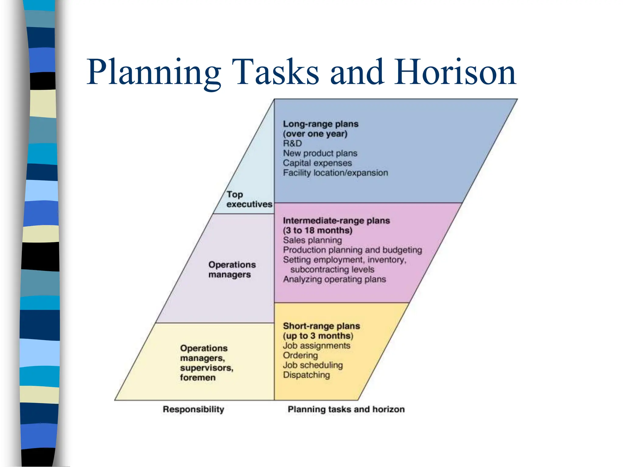
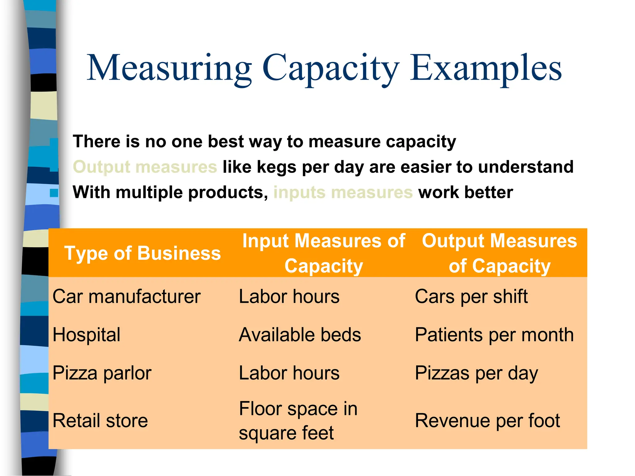
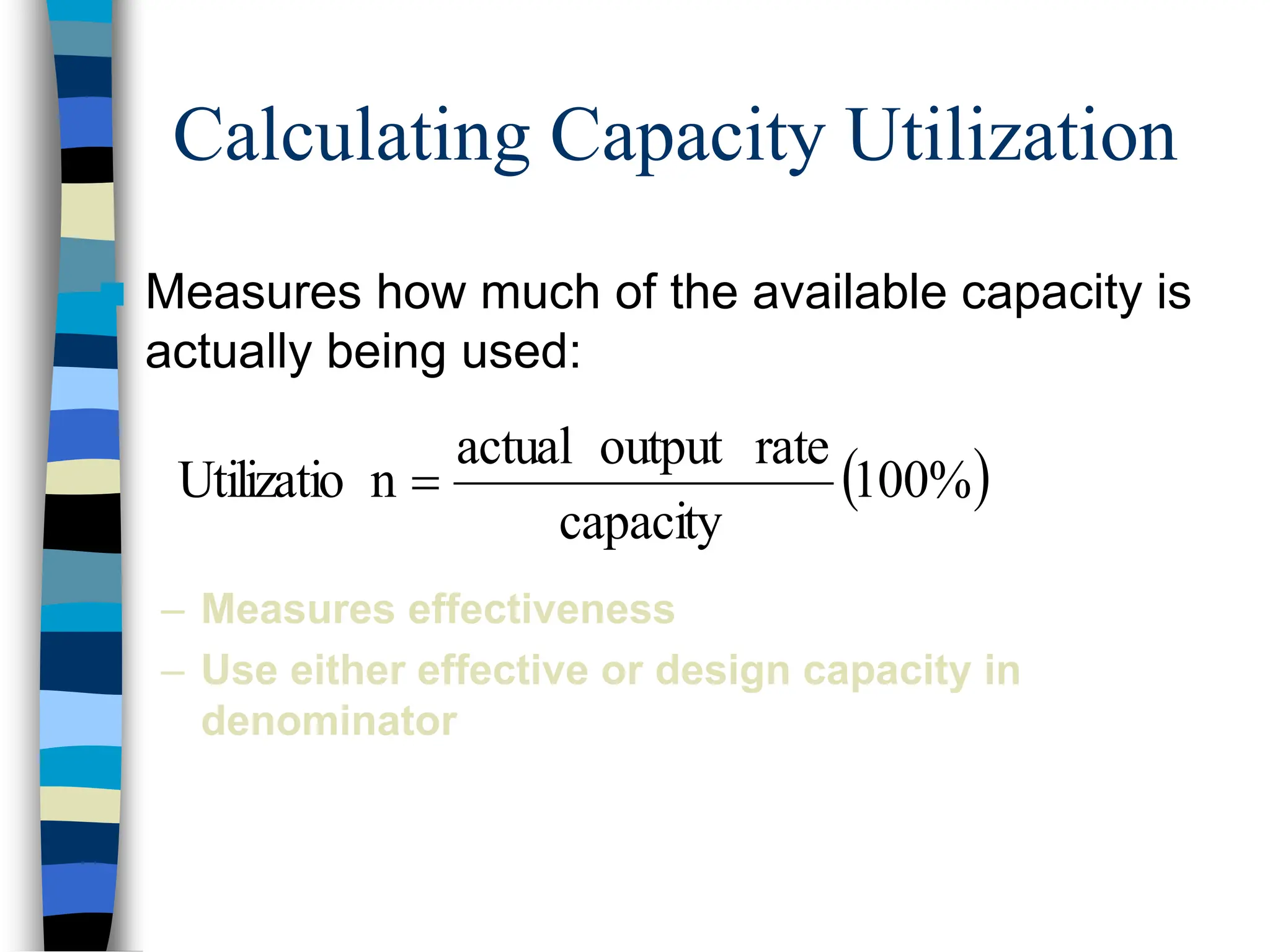
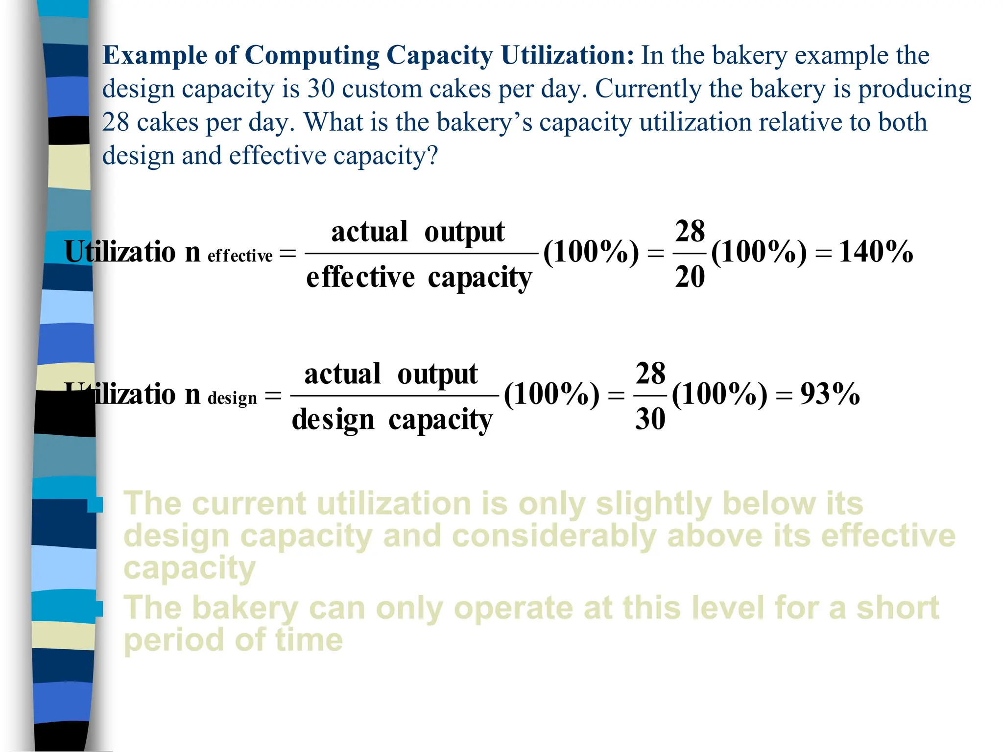
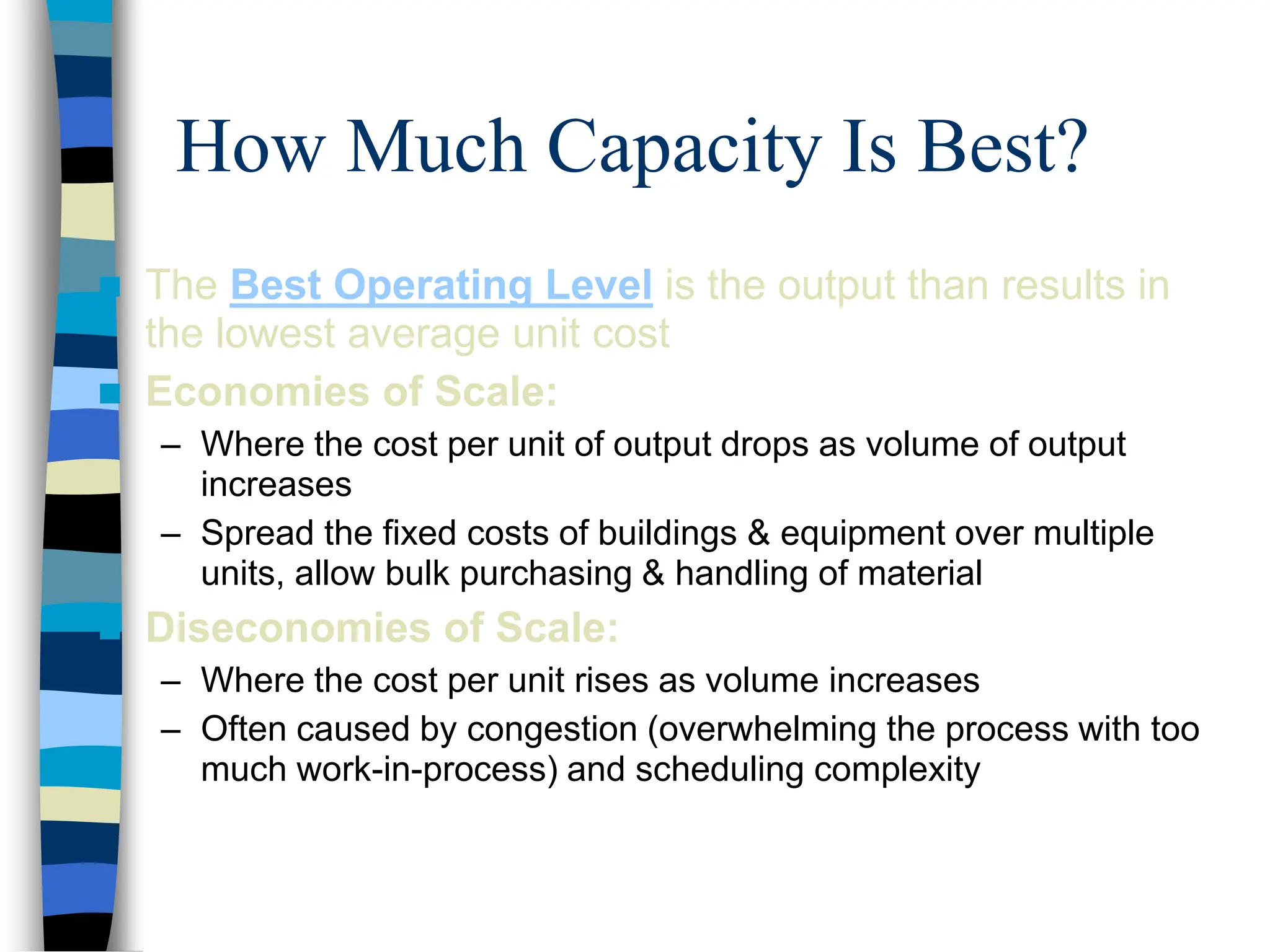
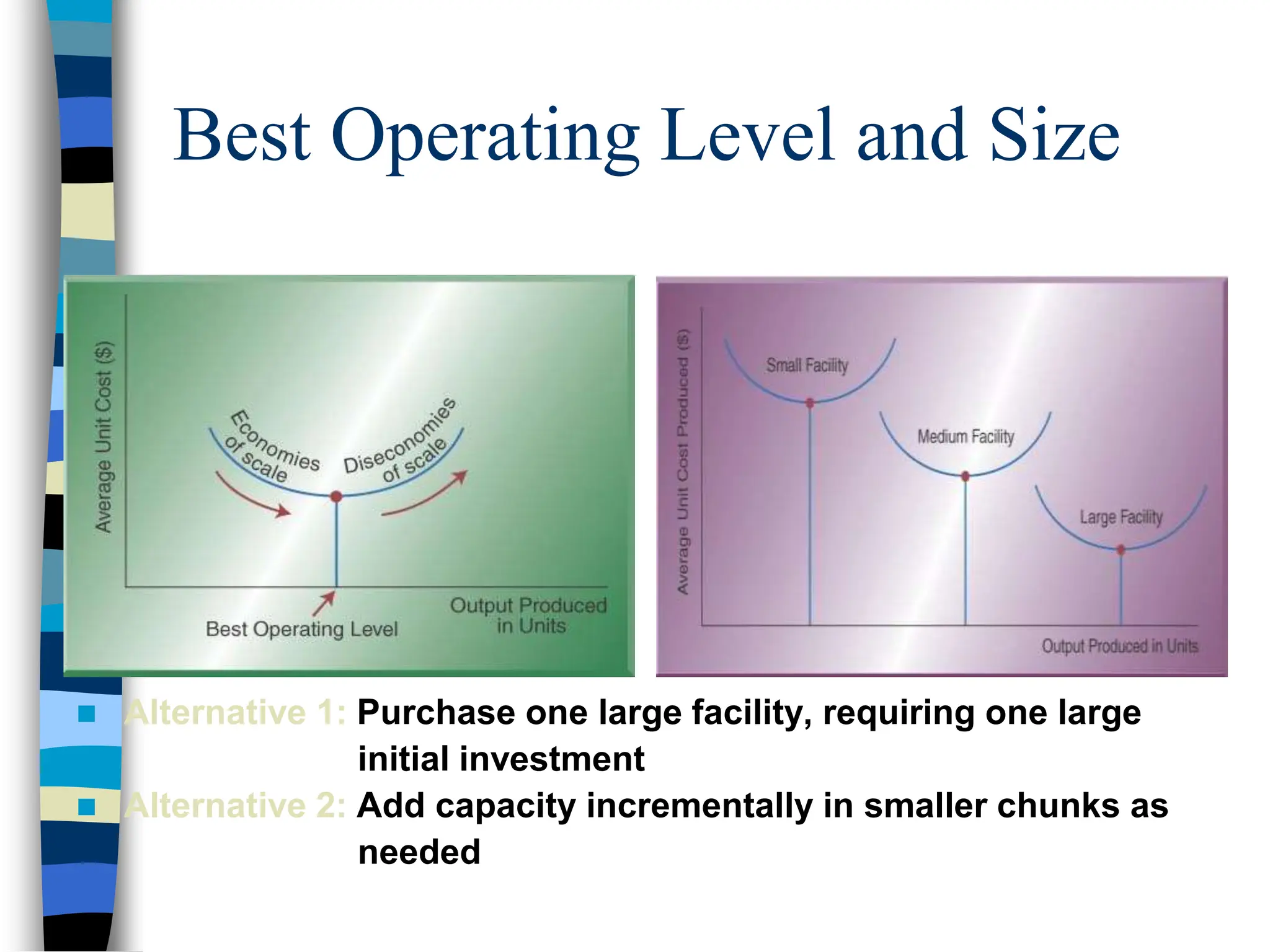
Aggregate Planning for industrial engineering

Capacity planning
 Capacity is the maximum output rate of a
production or service facility
 Capacity planning is the process of establishing
the output rate that may be needed at a facility:
– Capacity is usually purchased in “chunks”
– Strategic issues: how much and when to
spend capital for additional facility &
equipment
– Tactical issues: workforce & inventory levels, &
day-to-day use of equipment

Measuring Capacity Examples
 There is no one best way to measure capacity
 Output measures like kegs per day are easier to understand
 With multiple products, inputs measures work better
Type of Business
Input Measures of
Capacity
Output Measures
of Capacity
Car manufacturer Labor hours Cars per shift
Hospital Available beds Patients per month
Pizza parlor Labor hours Pizzas per day
Retail store
Floor space in
square feet
Revenue per foot

Capacity Information Needed
 Design capacity:
– Maximum output rate under ideal
conditions
– A bakery can make 30 custom cakes per
day when pushed at holiday time
 Effective capacity:
– Maximum output rate under normal
(realistic) conditions
– On the average this bakery can make 20
custom cakes per day

Calculating Capacity Utilization
 Measures how much of the available capacity is
actually being used:
– Measures effectiveness
– Use either effective or design capacity in
denominator
 
100%
capacity
rate
output
actual
n
Utilizatio 

Example of Computing Capacity Utilization: In the bakery example the
design capacity is 30 custom cakes per day. Currently the bakery is producing
28 cakes per day. What is the bakery’s capacity utilization relative to both
design and effective capacity?
93%
(100%)
30
28
(100%)
capacity
design
output
actual
n
Utilizatio
140%
(100%)
20
28
(100%)
capacity
effective
output
actual
n
Utilizatio
design
effective






 The current utilization is only slightly below its
design capacity and considerably above its effective
capacity
 The bakery can only operate at this level for a short
period of time

How Much Capacity Is Best?
 The Best Operating Level is the output than results in
the lowest average unit cost
 Economies of Scale:
– Where the cost per unit of output drops as volume of output
increases
– Spread the fixed costs of buildings & equipment over multiple
units, allow bulk purchasing & handling of material
 Diseconomies of Scale:
– Where the cost per unit rises as volume increases
– Often caused by congestion (overwhelming the process with too
much work-in-process) and scheduling complexity

Best Operating Level and Size
 Alternative 1: Purchase one large facility, requiring one large
initial investment
 Alternative 2: Add capacity incrementally in smaller chunks as
needed

Implementing Capacity
Decisions
 Capacity flexibility
– Plant, process, workers, outsourcing
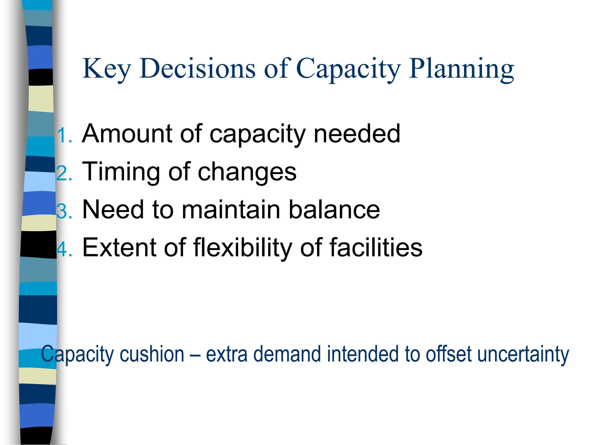
 Amount of capacity cushion
– important in -to-order and services
 Timing the capacity change
– Leading [proactive]
– Concurrent [neutral]
– Lagging [reactive]
 Size of the capacity increment

Making Capacity Planning Decisions
 The three-step procedure for making
capacity planning decisions is as
follows:
– Step 1: Identify Capacity Requirements
– Step 2: Develop Capacity Alternatives
– Step 3: Evaluate Capacity Alternatives

Evaluating Capacity Alternatives
 Could do nothing, or expand large now, or
expand small now with option to add later
 Use Decision Trees analysis tool:
– A modeling tool for evaluating sequential
decisions
– Identify the alternatives at each point in time
(decision points), estimate probable consequences
of each decision (chance events) & the ultimate
outcomes (e.g.: profit or loss)

Efficiency and Utilization
Actual output
Efficiency =
Effective capacity
Actual output
Utilization =
Design capacity
Both measures expressed as percentages

Efficiency/Utilization Example
Actual output = 36 units/day
Efficiency = =
90%
Effective capacity 40 units/ day
Utilization = Actual output = 36 units/day
=
72% Design capacity 50 units/day
Design capacity = 50 trucks/day
Effective capacity = 40 trucks/day
Actual output = 36 units/day

90.00%
72.00%
0.00%
10.00%
20.00%
30.00%
40.00%
50.00%
60.00%
70.00%
80.00%
90.00%
100.00%
Efficiency Utilization
Efficiency vs Utilization

Utilization Example
 Best operating level = 120 units/week
 Actual output = 83 units/week
 Utilization = ?
.692
units/wk
120
units/wk
83
=
level
operating
Best
used
Capacity
n
Utilizatio 


Actual production last week = 148,000 rolls
Effective capacity = 175,000 rolls
Design capacity = 1,200 rolls per hour
Bakery operates 7 days/week,
Shifts/day = 3,
Hours/shift = 8
Design capacity = (7 x 3 x 8) x (1,200)
= 201,600 rolls/week
Measuring capacity
Ex.
Utilization = 148,000/201,600 = 73.4%
Efficiency = 148,000/175,000 = 84.6%

 Facilities (size, location, layout, heating, lighting, ventilations)
 Product and service factors (similarity of products)
 Process factors (productivity, quality)
 Human factors (training, skills, experience, motivations,
absentation, turnover)
 Policy factors (overtime system, no. of shifts)
 Operational factors (scheduling problems, purchasing
requirements, inventory shortages)
 Supply chain factors (warehousing, transportation,
distribution)
 External factors (product standards, government agencies,
pollution standard)
Determinants of Effective Capacity

Estimate future capacity requirements
Evaluate existing capacity
Identify alternatives
Conduct financial analysis for each alt.
Assess key qualitative issues for each alt.
Select one alternative
Implement alternative chosen
Monitor results
Steps for Capacity Planning

Calculating Processing
Requirements
Determine type of products or services
Forecast for the Demand
Determine the process requirements
•The standard processing time / unit of
product
•The number of workdays / year
•The number shifts that will be used

Product
Annual
Demand
Standard
processing time
per unit (hr.)
Processing time
needed (hr.)
#1
#2
#3
400
300
700
5.0
8.0
2.0
2,000
2,400
1,400
5,800
Calculating Processing Requirements
A dept. works 8-hour shift, 250 days/year
annual capacity is 250*8 = 2000 hours,
number of machines required = 5,800 hours/2,000 hours = 2.90 machines
then we need three machines to handle the required volume

In-House or Outsourcing
1. Available capacity (equip.,skills,time)
2. Expertise
3. Quality considerations (labs, inspect.)
4. Nature of demand (high, steady)
5. Cost (fixed, savings)
6. Risk
Outsource: obtain a good or service completely or partially
from an external provider
Make or Buy ?

A firm’s manager must decide whether to make or buy a
certain item used in the production of vending machines ,
making the item would involve annual lease costs of
$150000 . Cost and volume estimates are as follows:
•Should the firm make or buy ?
•If the volume changed , at what volume would the
manager be indifferent between making and buying ?
Buy
Make
None
$150000
Annual fixed cost
$80
$60
Variable cost/unit
12000
12000
Annual volume (units)
EX.
Make or Buy ?

• Total cost = Fixed cost + (Volume * Variable cost)
in case of make = $150000 + (12000*60) = $870000
in case of buy = 0 + (12000*80) = $960000
TCost (make) < TCost (buy)
So the solution is “Make”
• Tcost(make) = Tcost(buy)
$150000 + Q*60 = 0 + Q*80
Q = 7500 unit
Sol.
Make or Buy ?
Q

Determinants of Effective Capacity
• Facilities
• Product and service factors
• Process factors ( output quality )
• Human factors
• Operational factors ( late delivery
for the raw materials )
• Supply chain factors
• External factors

Key Decisions of Capacity Planning
1. Amount of capacity needed
2. Timing of changes
3. Need to maintain balance
4. Extent of flexibility of facilities
Capacity cushion – extra demand intended to offset uncertainty

Steps for Capacity Planning
1. Estimate future capacity requirements
2. Evaluate existing capacity
3. Identify alternatives
4. Conduct financial analysis
5. Assess key qualitative issues
6. Select one alternative
7. Implement alternative chosen
8. Monitor results

Make or Buy
1. Available capacity
2. Expertise
3. Quality considerations
4. Nature of demand
5. Cost
6. Risk

Example 3
• A manager must decide which type of equipment
to buy , type A or type B. type A equipment costs
$15000 each and type B costs $ 11000. the
equipment can be operated 8 hours a day ,250
days a year.
• Either machine can be used to perform two types
of chemical analysis C1 and C2 annual service
requirement and processing times are shown in
the following table.
• Which type of equipment should be purchased
and how many of that type will be need ? The
goal is to minimize total purchase cost.

Total processing time ( annual volume × processing time per analysis ) needed by
type of equipment.
Processing
time per
analysis ( HR)
Processing
time per
analysis ( HR)
Analysis type Annual volume A B
C1
C2
1200
900
1
3
2
2
Analysis type A B
C1
C2
1200
2700
2400
1800
3900 4200

Solution:
• Total processing time available per price of
equipment is 8 hours/day × 250 days/year
=2000
• Hence , one piece can handle 2000 hours of
analysis ,two pieces of equipment can handle
4000 hours and so on.
• Given the total processing requirement two of
type A would be needed for a total cost of 2 ×
15000=30000 or three of type B for a total cost of
3× 11000=33000 thus two pieces of type A would
have sufficient capacity to Handle the load at
lower cost than three of type B

Planning Service Capacity
 Need to be near customers
– Capacity and location are closely tied
 Inability to store services
– Capacity must be matched with timing of
demand
 Degree of volatility of demand
– Peak demand periods

Assumptions of Cost-Volume
Analysis
1. One product is involved
2. Everything produced can be sold
3. Variable cost per unit is the same
regardless of volume
4. Fixed costs do not change with volume
5. Revenue per unit constant with volume
6. Revenue per unit exceeds variable cost
per unit

Financial Analysis
 Cash Flow - the difference between
cash received from sales and other
sources, and cash outflow for labor,
material, overhead, and taxes.
 Present Value - the sum, in current
value, of all future cash flows of an
investment proposal.

 Meet demand
(Sales Forecast)
 Use capacity efficiently
 Meet inventory policy
 Minimize cost
– Labor
– Inventory
– Plant & equipment
– Subcontract
Aggregate Planning Goals

Aggregate Planning Strategies
Pure Strategies
Demand Options — change demand:
 influencing demand (e.g. change price)
 backordering during high demand periods
 counterseasonal product mixing

Pure Strategies
Capacity Options — change capacity:
 changing inventory levels
 varying work force size by hiring or layoffs
 varying production capacity through
overtime or idle time
 subcontracting (aka “outsourcing”)
 using part-time workers

Aggregate Scheduling Options -
Advantages and Disadvantages
Option Advantage Disadvantage Some
Comments
Changing
inventory levels
Changes in
human resources
are gradual, not
abrupt
production
changes
Inventory
holding costs;
Shortages may
result in lost
sales
Applies mainly
to production,
not service
operations
Varying
workforce size
by hiring or
layoffs
Avoids use of
other alternatives
Hiring, layoff,
and training
costs
Used where size
of labor pool is
large

Comments
Varying
production rates
through overtime
or idle time
Matches seasonal
fluctuations
without
hiring/training
costs
Overtime
premiums, tired
workers, may not
meet demand
Allows
flexibility within
the aggregate
plan
Subcontracting Permits
flexibility and
smoothing of the
firm's output
Loss of quality
control; reduced
profits; loss of
future business
Applies mainly
in production
settings
Advantages/Disadvantages -
continued

Advantages/Disadvantages -
continued
Comments
Using part-time
workers
Less costly and
more flexible
than full-time
workers
High
turnover/training
costs; quality
suffers;
scheduling
difficult
Good for
unskilled jobs in
areas with large
temporary labor
pools
Influencing
demand
Tries to use
excess capacity.
Discounts draw
new customers.
Uncertainty in
demand. Hard to
match demand to
supply exactly.
Creates
marketing ideas.
Overbooking
used in some
businesses.

Advantage/Disadvantage -
continued
Comments
Back ordering
during high-
demand periods
May avoid
overtime. Keeps
capacity constant
Customer must
be willing to
wait, but
goodwill is lost.
Many companies
backlog.
Counterseasonal
products and
service mixing
Fully utilizes
resources; allows
stable workforce.
May require
skills or
equipment
outside a firm's
areas of
expertise.
Risky finding
products or
services with
opposite demand
patterns.

The Extremes
Level
Strategy
Chase
Strategy
Production
equals sales
forecast
Production rate
is constant

 Level scheduling strategy
– Produce same amount every day
– Keep work force level constant
– Vary non-work force capacity or demand options
– Often results in lowest production costs
 Chase scheduling strategy
– Vary the amount of production to match (chase) the
sales forecast
– This requires changing the workforce (hiring & firing)
 Mixed strategy
– Combines 2 or more aggregate scheduling options

The Trial & Error Approach to
Aggregate Planning
 Forecast the demand for each period
 Determine the capacity for regular time,
overtime, and subcontracting, for each
period
 Determine the labor costs, hiring and firing
costs, and inventory holding costs
 Consider company policies which may
apply to the workers, overtime,
outsourcing, or to inventory levels
 Develop alternative plans, and examine
their total costs

The IDES Sales Forecast for 2003
Unit Sales Forecast
For 2003
Quarter 1 307,200
Quarter 2 379,200
Quarter 3 360,000
Quarter 4 489,600
Total 1,536,000

IDES Manufacturing Example
 IDES Manufacturing wants to compare the
annual (year 2003) costs associated with
scheduling using the following three (3)
options:
 Option 1 – Maintain a constant work force
during the entire year (Level).
 Option 2 – Maintain the present work force of
150 and use overtime and sub-contracting as
needed (Mixed)
 Option 3 – Hire/layoff workers as needed to
produce the required output (Chase).

IDES Cost Information
 Inventory Carrying Cost
(per quarter) $ 0.50/unit
 Subcontracting cost $ 7/unit
 Pay rate – regular time $20/hr
 Pay rate – overtime $30/hr
 Labor standard per unit 0.2 hrs
 Cost to increase production $ 3/unit
 Cost to decrease production $ 2/unit
 IDES has 0 units in inventory
 Each Quarter has 60 working days
 At end of 2002, IDES has 150 prod. workers
 IDES Policy – Maximum of 72,000 units/qtr produced
using overtime

Option 1 – Constant Workforce
without overtime or subcontracting
 First, determine the number of workers
required to produce the units forecast for
2003.
 Ave. Prod/day = 1,536,000 = 6,400/day
240 days
 Then determine how many workers are
needed.
 Workers needed = 6,400/day = 160
5 units/hr X 8 hrs

Option 1 Continued:
Calculate Inventory Carrying Costs
Qtr Production
@ 6400/day
Sales
Forecast
Inventory
Change
Ending
Inventory
1 384,000 307,200 +76,800 76,800
2 384,000 379,200 + 4,800 81,600
3 384,000 360,000 +24,000 105,600
4 384,000 489,600 -105,600 0
Total 1,536,000 1,536,000 264,000

Option 1 Continued:
Calculation of Annual Costs
 Inventory carrying cost:
264,000 units X $0.50/unit = $ 132,000
 Cost to increase capacity:
(384,000-360,000) units X $5/unit = $ 120,000
 Regular time labor cost:
1,536,000 units X $4/unit = $6,144,000
 Total Annual Cost for Option 1 = $6,396,000

Option 2 – Present Workforce (150) using
O/T & subcontracting
Qtr Sales
Forecast
In-house
Production
Inv
Change
End
Inv
Units
Req’d
O/T Out
Source
1 307,200 360,000 +52,800 52,800 0 0 0
2 379,200 360,000 -19,200 33,600 0 0 0
3 360,000 360,000 0 33,600 0 0 0
4 489,600 360,000 -33,600 0 96,000 72,000 24,000
Tot
al
1,536,000 1,440,000 0 72,000 24,000

Option 2 Continued:
 Inventory Carrying Costs
120,000 units X $.50/unit = $ 60,000
 Regular time labor (150 workers)
$4/unit X 1,440,000 units = $5,760,000
 Overtime labor
$6/unit X 72,000 units = $ 432,000
 Out-sourcing
$7/unit X 24,000 units = $ 168,000
 Total Annual Costs for Option 2 = $6,420,000

Option 3 – Vary Production
(Workforce) to match Sales Forecast
Qtr
Sales
Forecast
Beginning
Capacity
Capacity
Change
Needed
Cost of
Capacity
Change
1 307,200 360,000 -52,800 $105,600
2 379,200 307,200 +72,000 216,000
3 360,000 379,200 -19,200 38,400
4 489,600 360,000 +129,600 388,800
Total 1,536,000 $748,800

Option 3 Continued
 Regular time labor costs
1,536,000 units X $4/unit = $6,144,000
 Capacity Change Costs = $ 748,800
 Total Annual Cost - Option 3 = $6,892,800

Annual Cost Comparison of the
Aggregate Scheduling Strategies
Option Annual Cost
1. Level – No use of O/T or
Outsourcing
$6,396,000
2. Mixed – Present work
force w/ O/T & Outsourcing
$6,420,000
3. Chase – Vary Production
(workforce)
$6,892,800

Homework Problem – Due at the
beginning of class Tuesday March 11
 Use the Revised IDES Cost information
shown on the following two slides to
evaluate the following scheduling
options:
 Level Strategy
 Chase Strategy
 Maintain Present work force and use
overtime production and sub-contracting
as needed

The IDES Sales Forecast for 2003
Revised
Unit Sales Forecast
For 2003
Quarter 1 388,000
Quarter 2 440,000
Quarter 3 400,000
Quarter 4 500,000
Total 1,728,000

IDES Cost Information - Revised
 Inventory Carrying Cost
(per quarter) $ 0.75/unit
 Subcontracting cost $ 7.50/unit
 Pay rate – regular time $20/hr
 Pay rate – overtime $30/hr
 Labor standard per unit 0.2 hrs
 Cost to increase production $ 1.50/unit
 Cost to decrease production $ 1/unit
 IDES has 0 units in inventory
 Each Quarter has 60 working days
 At end of 2000, IDES has 140 prod. workers
 IDES Policy – Maximum of 78,000 units/qtr produced
using overtime

Aggregate Planning for industrial engineering

Recommended

Recommended

More Related Content

Similar to Aggregate Planning for industrial engineering

Similar to Aggregate Planning for industrial engineering (20)

More from ashaby

More from ashaby (9)

Recently uploaded

Recently uploaded (20)

Aggregate Planning for industrial engineering