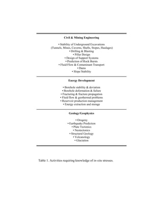
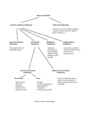
This document provides an overview of stresses and strains in rock mechanics. It discusses key topics such as:
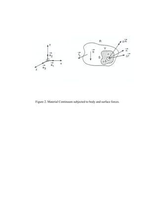
- The Cauchy stress principle which defines stress as a force per unit area.
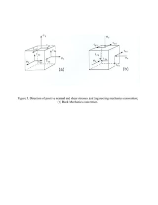
- Representing the state of stress at a point using stress tensors and describing normal stresses, shear stresses, and principal stresses.
- Transforming stresses between coordinate systems using stress transformation laws.
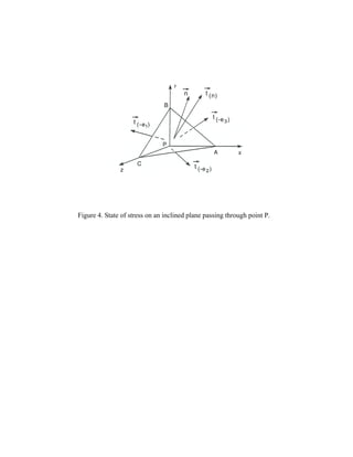
- Relating stresses on inclined planes to the stress tensor components.
- Equilibrium conditions for stresses and the symmetry of the stress tensor.
- Decomposing stresses into hydrostatic and deviatoric components and defining octahedral stresses.
The document also outlines strain analysis concepts such as deformation and strain

![CVEN 5768 - Lecture Notes 3 Page 6
© B. Amadei
(9)
(10)
(11)
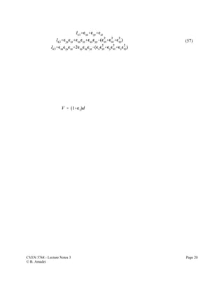
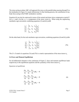
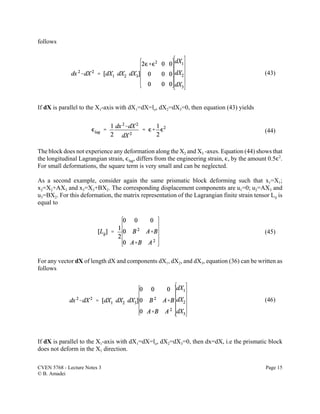
where D is the density and Db1, Db2 and Db3 are the components of the body force per unit volume
of the continuum in the x, y and z directions, respectively. The positive directions of those
components are in the positive x, y and z directions if the engineering mechanics convention for
stress is used, and in the negative x, y and z directions if the rock mechanics sign convention is used
instead.
Symmetry of stress tensor
which implies that only six stress components are needed to describe the state of stress at a point in
a continuum: three normal stresses and three shear stresses.
2.5 Stress Transformation Law
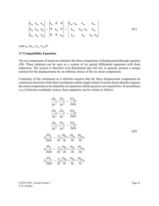
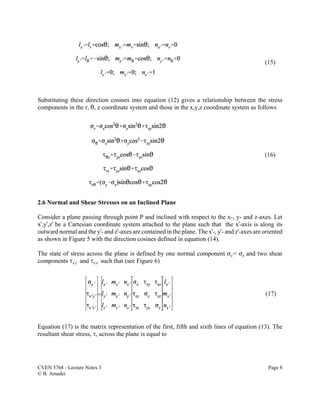
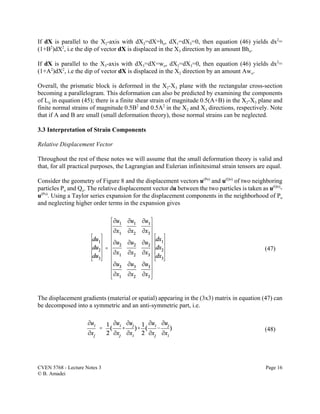
Consider now two rectangular coordinate systems x,y,z and xU,yU,zU at point P. The orientation of the
xU-, yU-, zU-axes is defined in terms of the direction cosines of unit vectors eU1, eU2 and eU3 in the x,y,z
coordinate system, i.e.
Let [A] be a coordinate transformation matrix such that
Matrix [A] is an orthogonal matrix with [A]t
= [A]-1
. Using the coordinate transformation law for
second order Cartesian tensors, the components of the stress tensor FUij in the xU,yU,zU coordinate
system are related to the components of the stress tensor Fij in the x,y,z coordinate system as follows](https://image.slidesharecdn.com/notes3-171104165057/85/Notes3-6-320.jpg)
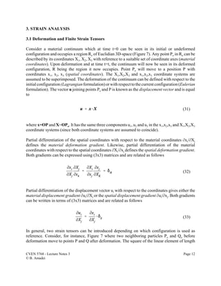
![CVEN 5768 - Lecture Notes 3 Page 7
© B. Amadei
(12)
(13)
(14)
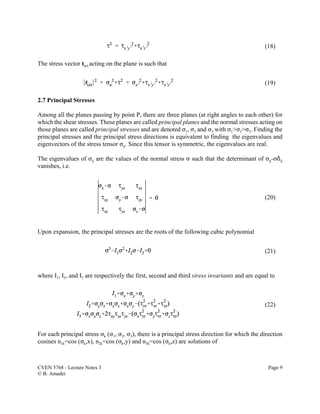
Using (6x1) matrix representation of FUij and Fij, and after algebraic manipulations, equation (12) can
be rewritten in matrix form as follows
where [F]t
xyz =[Fx Fy Fz Jyz Jxz Jxy], [F]t
x'y'z' =[FxU FyU FzU Jy'z' JxUzU JxUyU] and [TF] is a (6x6) matrix whose
components can be found in equation A1.23 in Goodman (1989). It can be written as follows
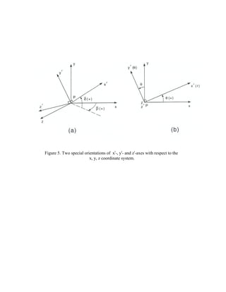
Expressions for the direction cosines lx', mx', nx'......are given below for two special cases shown in
Figures 5a and 5b, respectively. In Figure 5a, the orientation of the xU-axis is defined by two angles
$ and * and the zU-axis lies in the Pxz plane. In this case, the direction cosines are
If we take $=0, *=2, and the zU-axis to coincide with the z-axis, the xU-, yU- and zU-axes coincide, for
instance, with the radial, tangential and longitudinal axes of a cylindrical coordinate system r,2,z
(Figure 5b) with](https://image.slidesharecdn.com/notes3-171104165057/85/Notes3-7-320.jpg)
![CVEN 5768 - Lecture Notes 3 Page 18
© B. Amadei
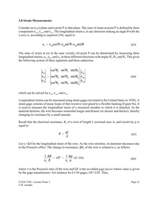
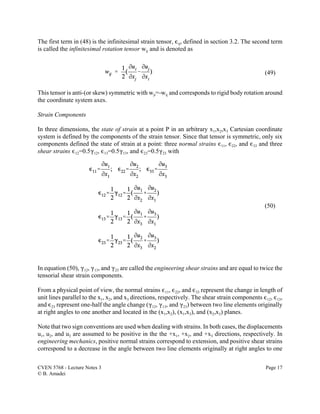
(51)
(52)
another. In rock mechanics, however, positive normal strains correspond to contraction (since
compressive stresses are positive), and positive shear strains correspond to an increase in the angle
between two line elements originally at right angles to one another. When using the rock mechanics
sign convention, the displacement components u1, u2, and u3 in equation (50) must be replaced by
-u1, -u2, and -u3, respectively.
3.4 Strain Transformation Law
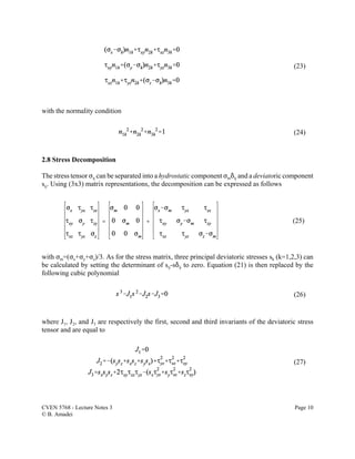
The components of the strain tensor ,Uij in an xU,yU,zU (x1U,x2U,x3U) Cartesian coordinate system can be
determined from the components of the strain tensor ,ij in an x,y,z (x1,x2,x3) Cartesian coordinate
system using the same coordinate transformation law for second order Cartesian tensors used in the
stress analysis. The direction cosines of the unit vectors parallel to the xU-,yU- and zU-axes are assumed
to be known and to be defined by equation (10). Equation (12) is replaced by
Using (6x1) matrix representation of ,Uij and ,ij, and after algebraic manipulations, equation (51) can
be rewritten in matrix form as follows
where [,]t
xyz =[,xx ,yy ,zz (yz (xz (xy], [,]t
x'y'z' =[,xUxU ,yUyU ,zUzU (y'z' (xUzU (xUyU] and [T,] is a (6x6) matrix with
components similar to those of matrix [TF] in equation (13). It can written as follows:](https://image.slidesharecdn.com/notes3-171104165057/85/Notes3-18-320.jpg)
![CVEN 5768 - Lecture Notes 3 Page 19
© B. Amadei
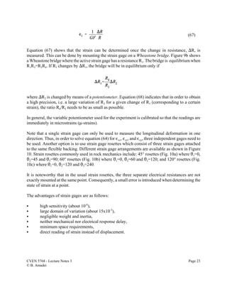
(53)
(54)
(55)
(56)
[TF] and [T,] are related as follows
Note that equation (53) is valid as long as engineering shear strains (and not tensorial shear strains)
are used in [,]xyz and [,]x'y'z'
The direction cosines defined in equation (15) can be used to determine the strain components in the
r, 2, z cylindrical coordinate system of Figure 5b. After algebraic manipulation, the strain
components in the r, 2, z and x,y,z coordinate systems are related as follows
3.5 Principal Strains
The principal strain values and their orientation can be found by determining the eigenvalues and
eigenvectors of the strain tensor ,ij. Equation (20) is replaced by
Upon expansion, the principal strains are the roots of the following cubic polynomial
where I,1, I,2, and I,3 are respectively the first, second and third strain invariants and are equal to](https://image.slidesharecdn.com/notes3-171104165057/85/Notes3-19-320.jpg)