Downloaded 13 times


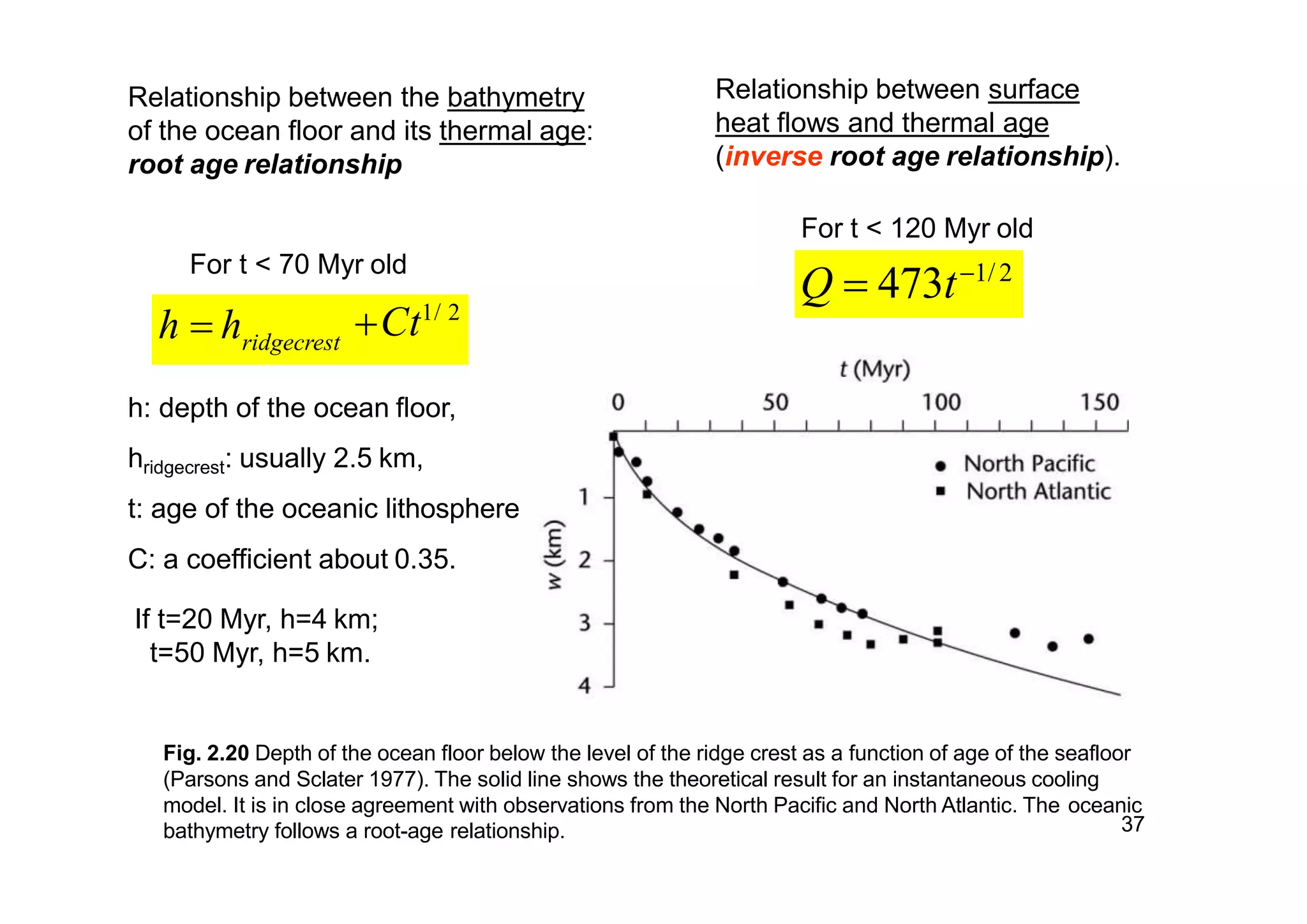
![Fig. 2.15 The dependence of the surface heat flow Q0 on the internal radiogenic heat production rate A
in a number of geological provinces. The intercept on the y-axis gives the so-called “reduced” heat flow
(20─30 mWm-2
). Derived from Roy et al. (1968), Turcotte and Schubert (2002). Reproduced courtesy
31of Cambridge University Press.
Granitic
terranes]
Reduced heat flows = mantle
heat flows
when there is no crustal
radiogenic heat production
(A=0).](https://image.slidesharecdn.com/2physicalstateofthelithosphere2010-181002170508/75/Physical-state-of-the-lithosphere-31-2048.jpg)


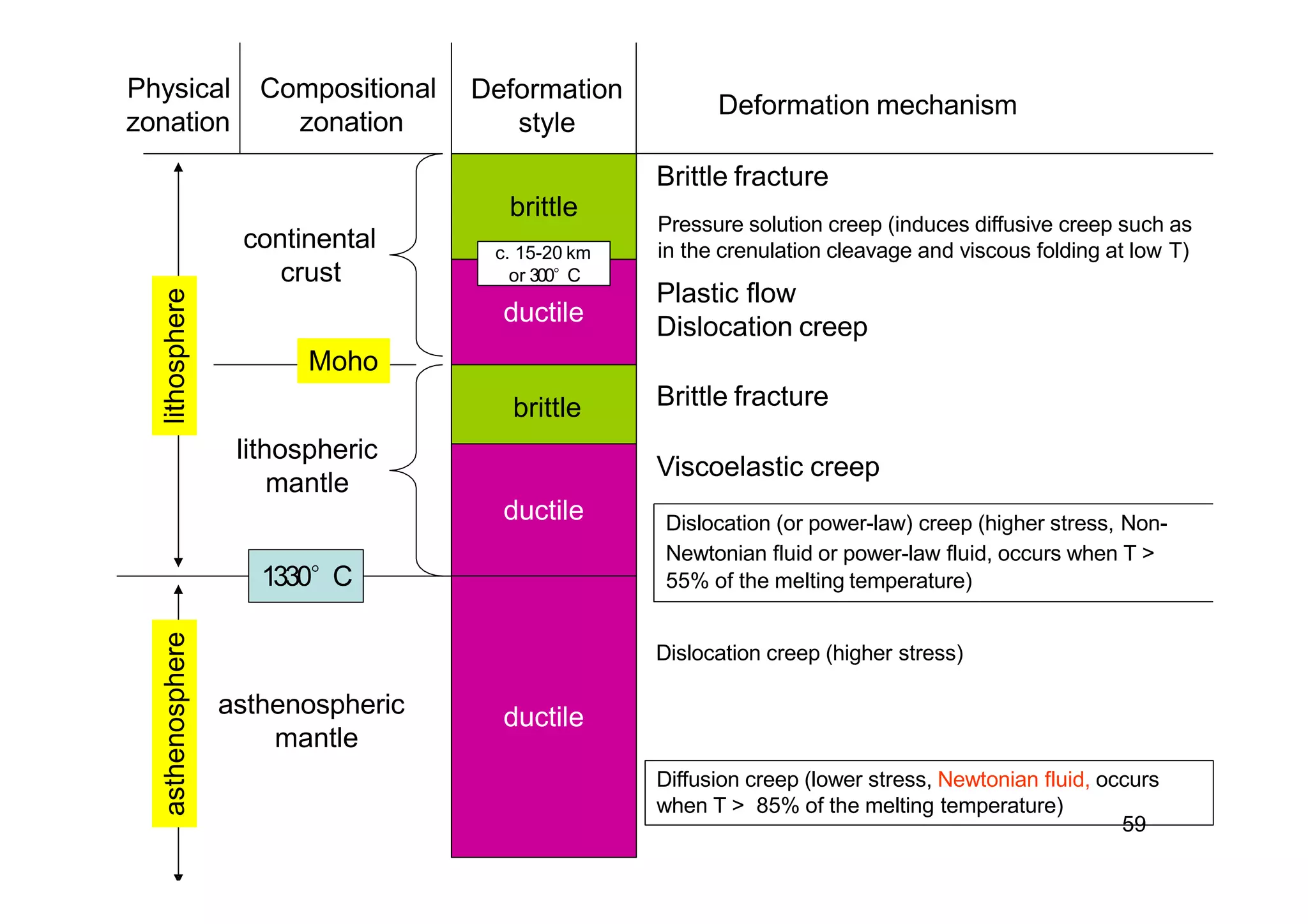

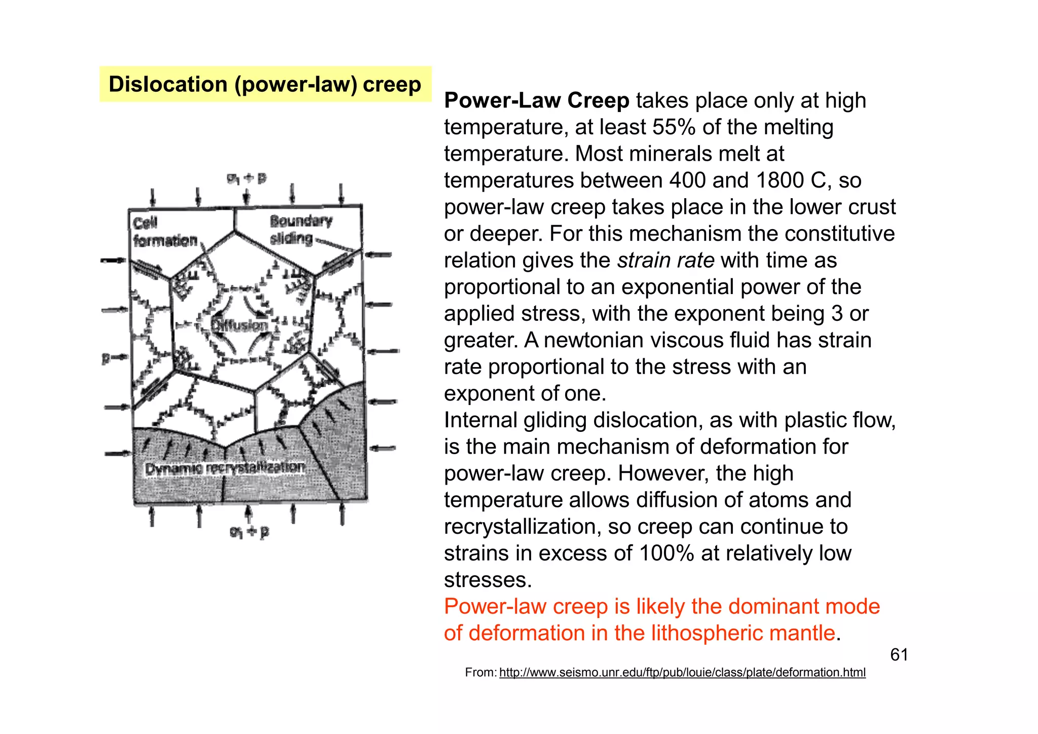

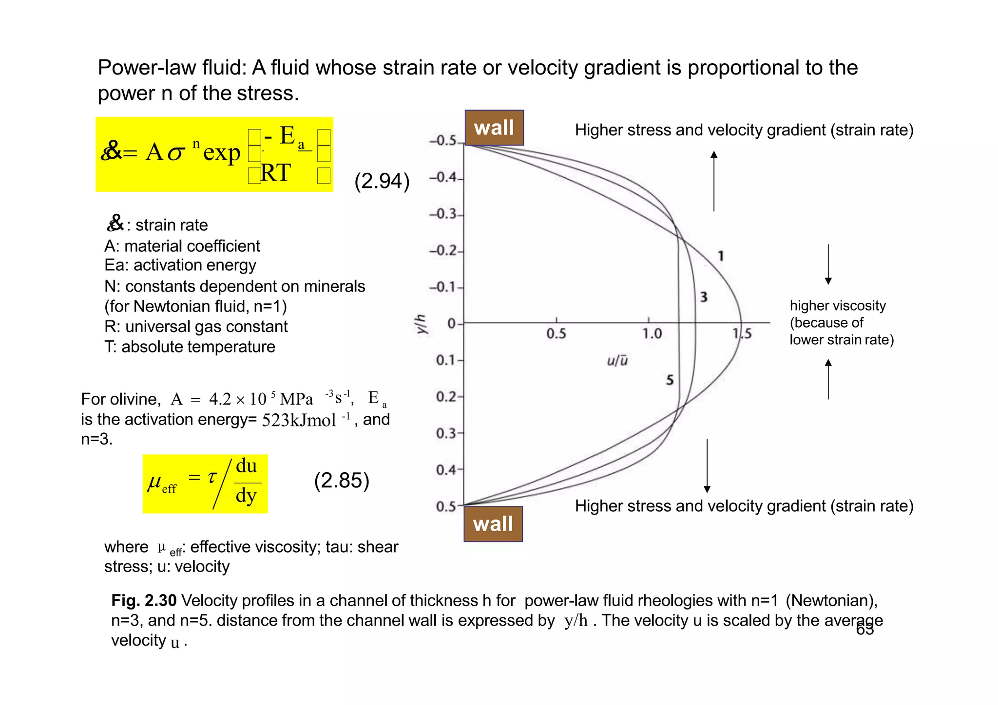
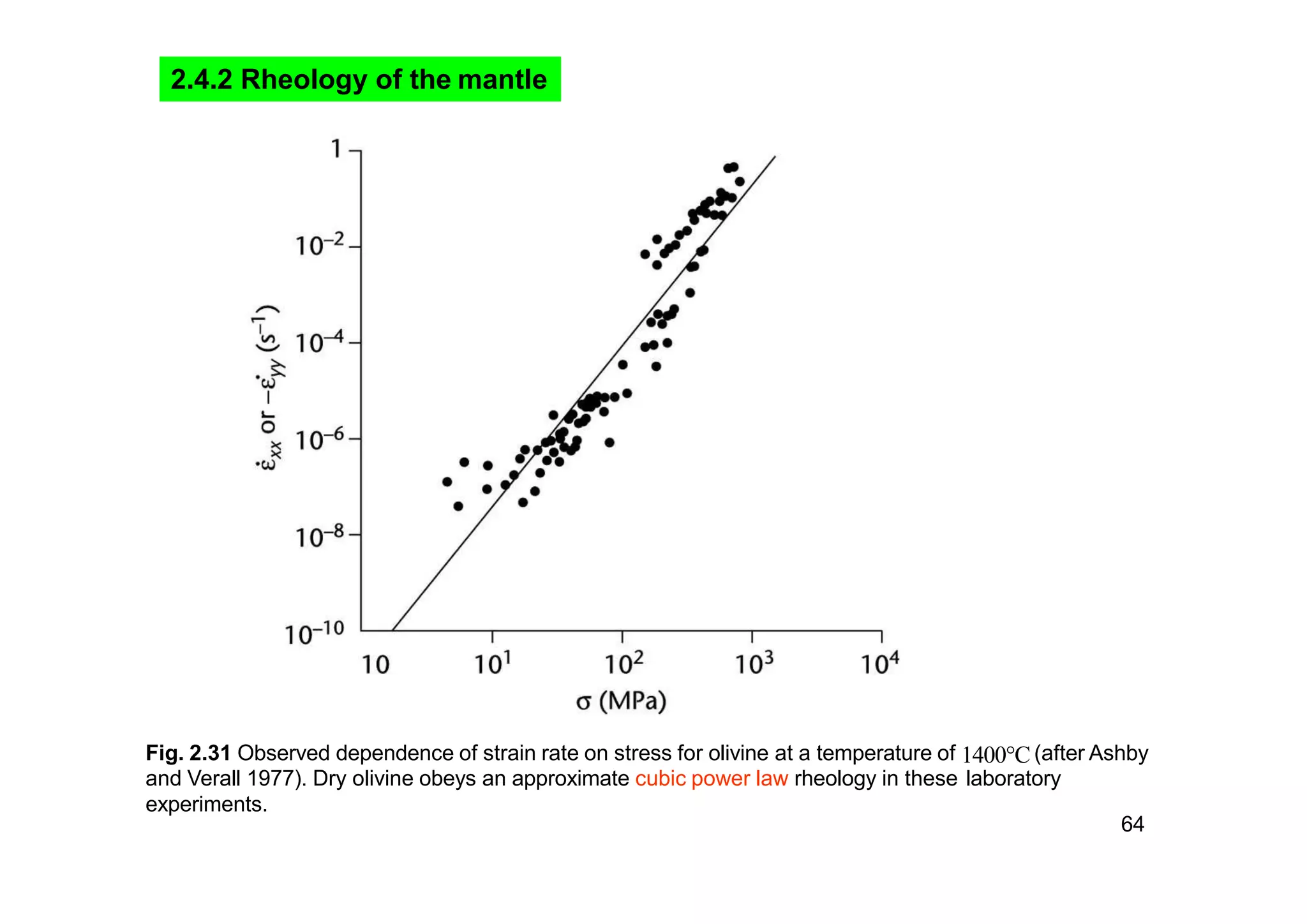


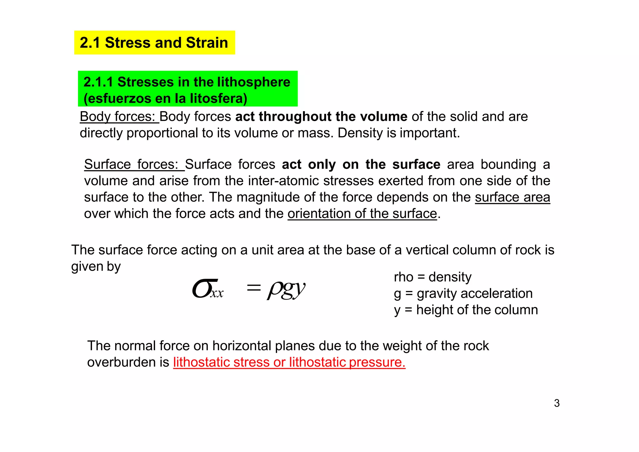
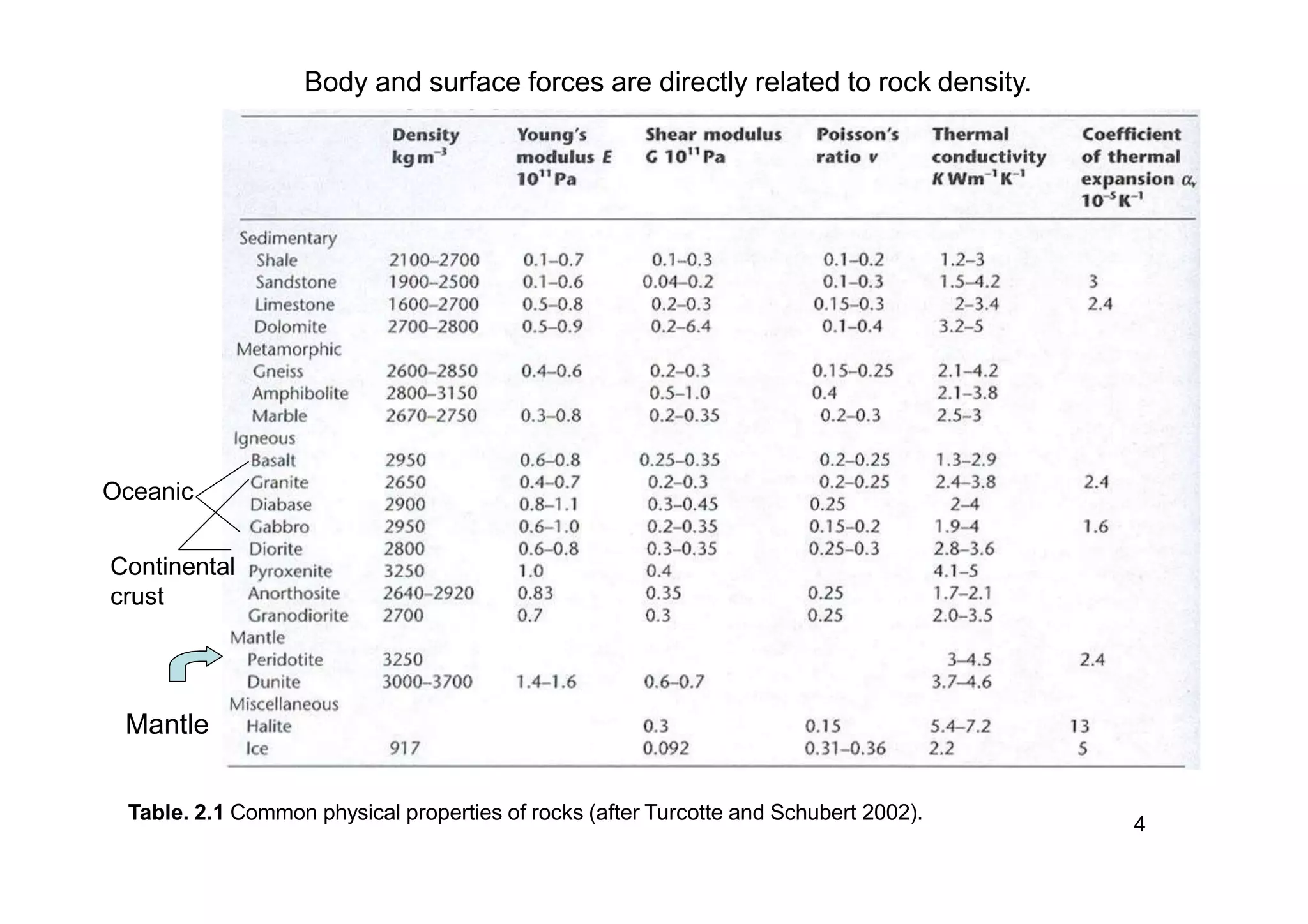
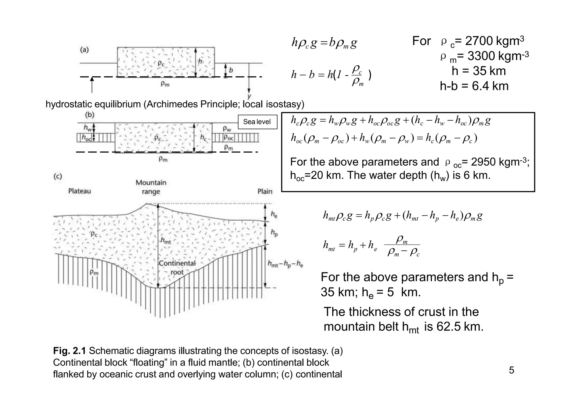
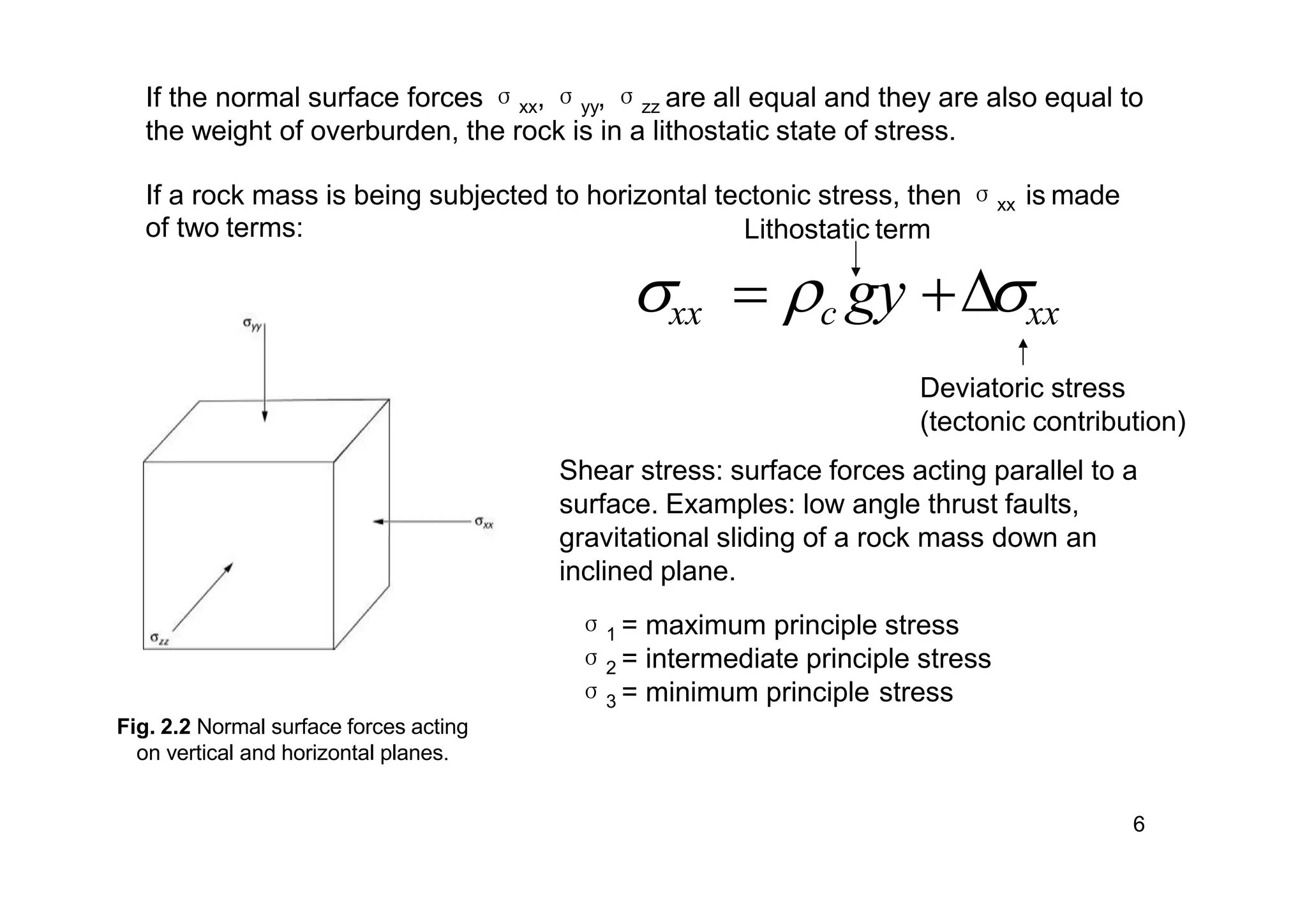
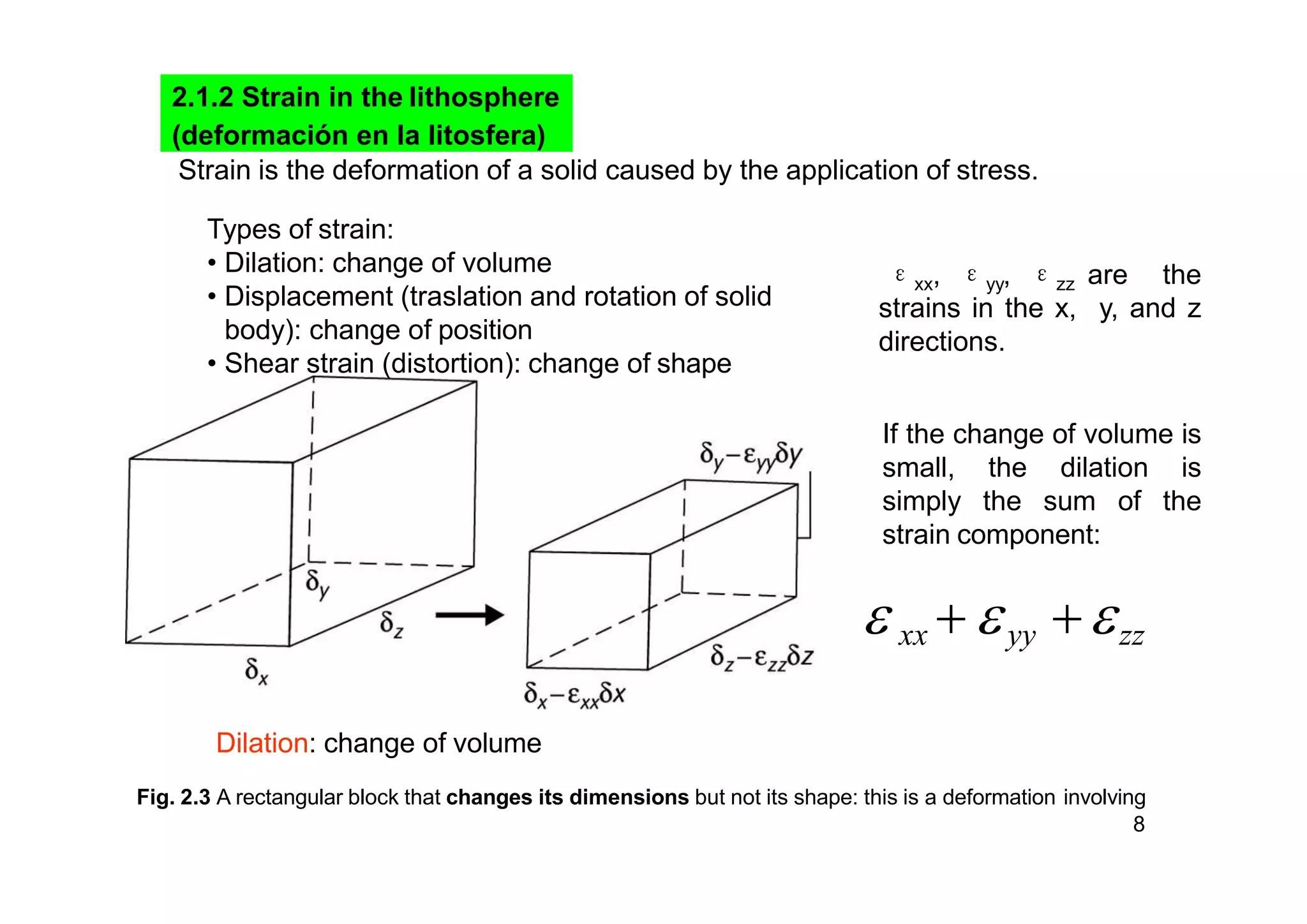
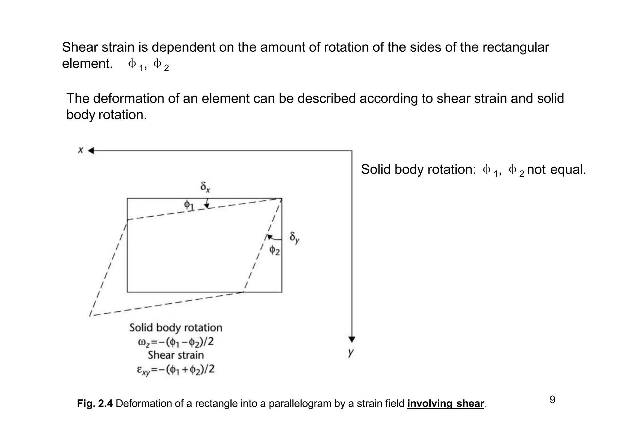
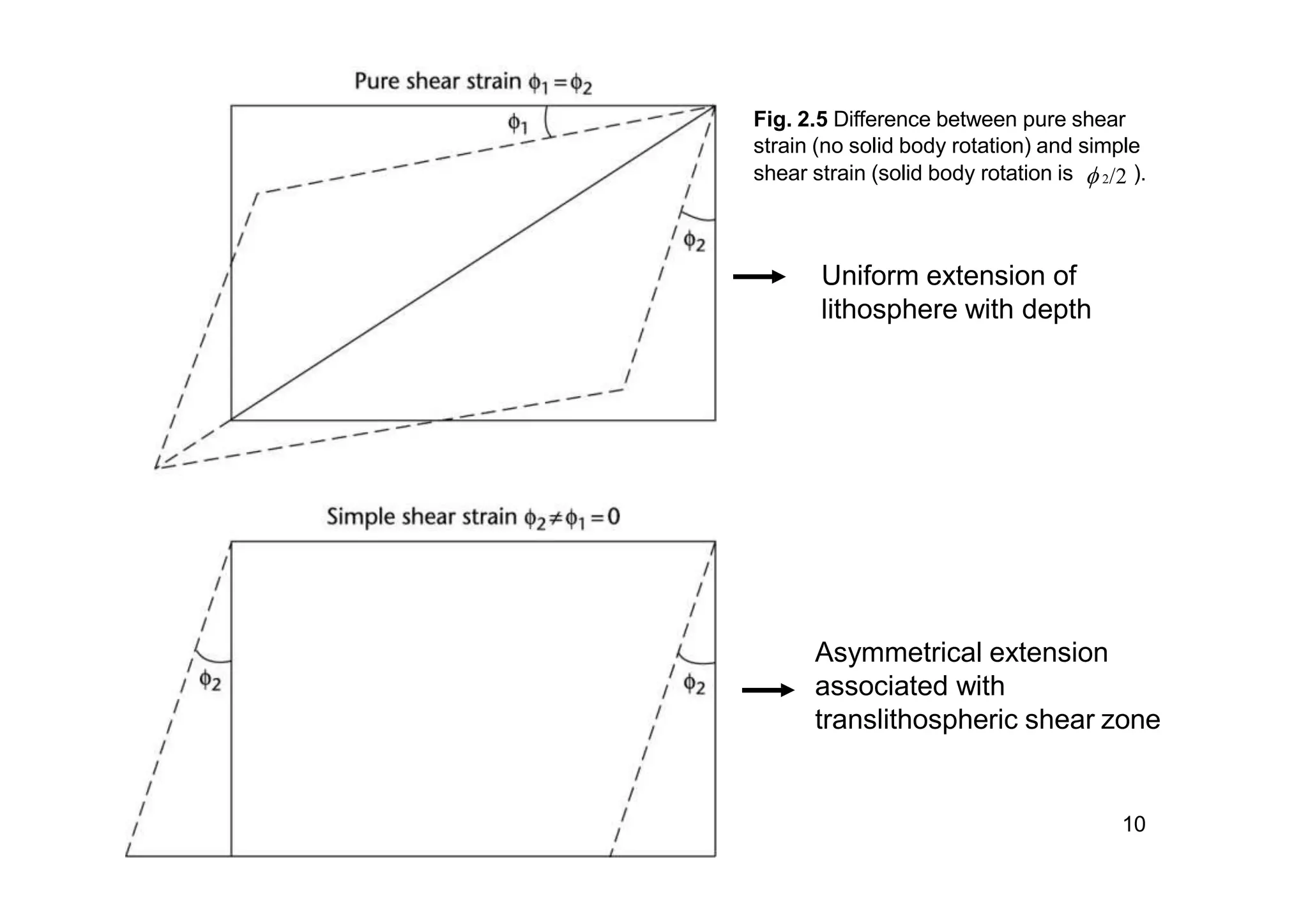
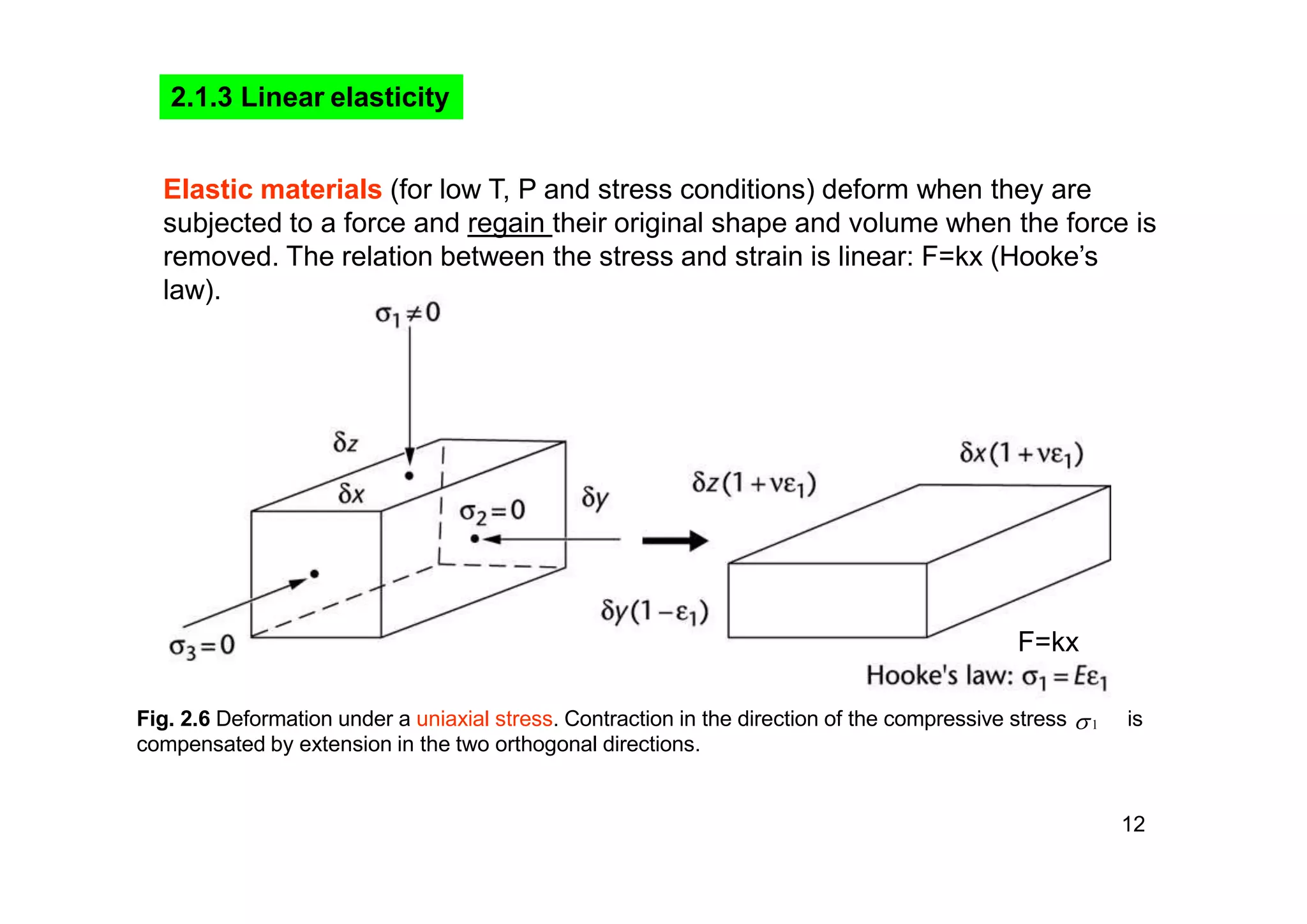
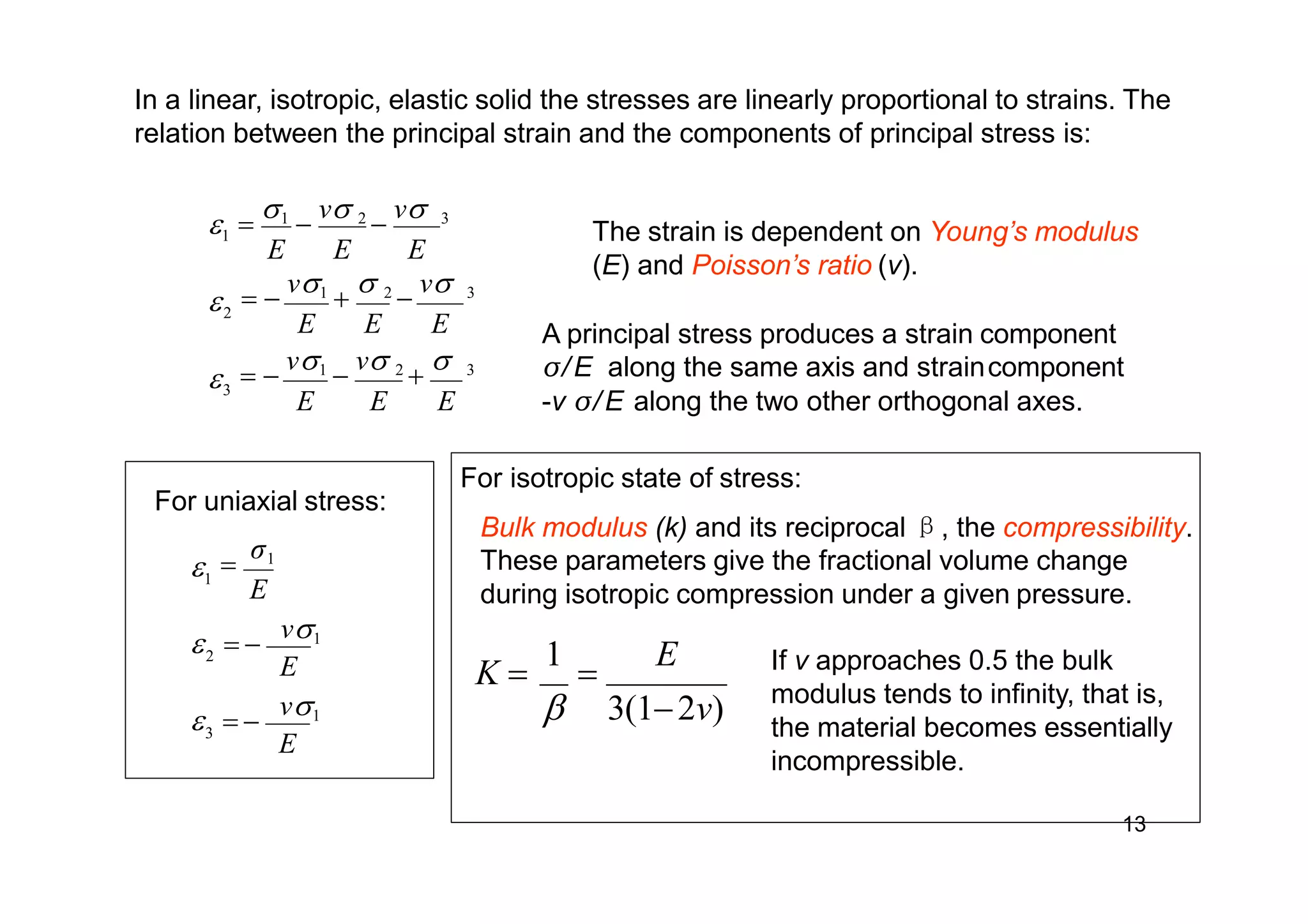
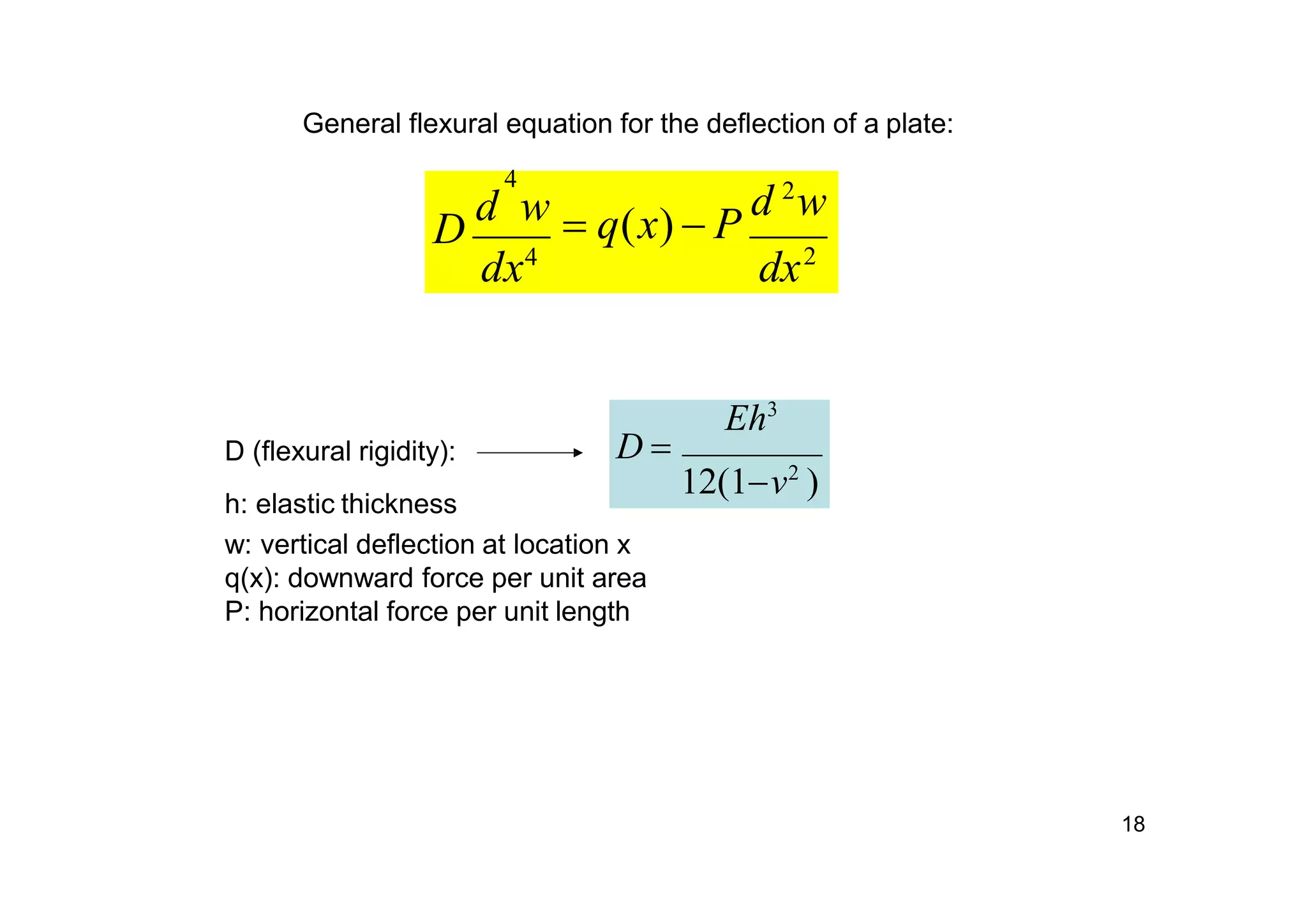
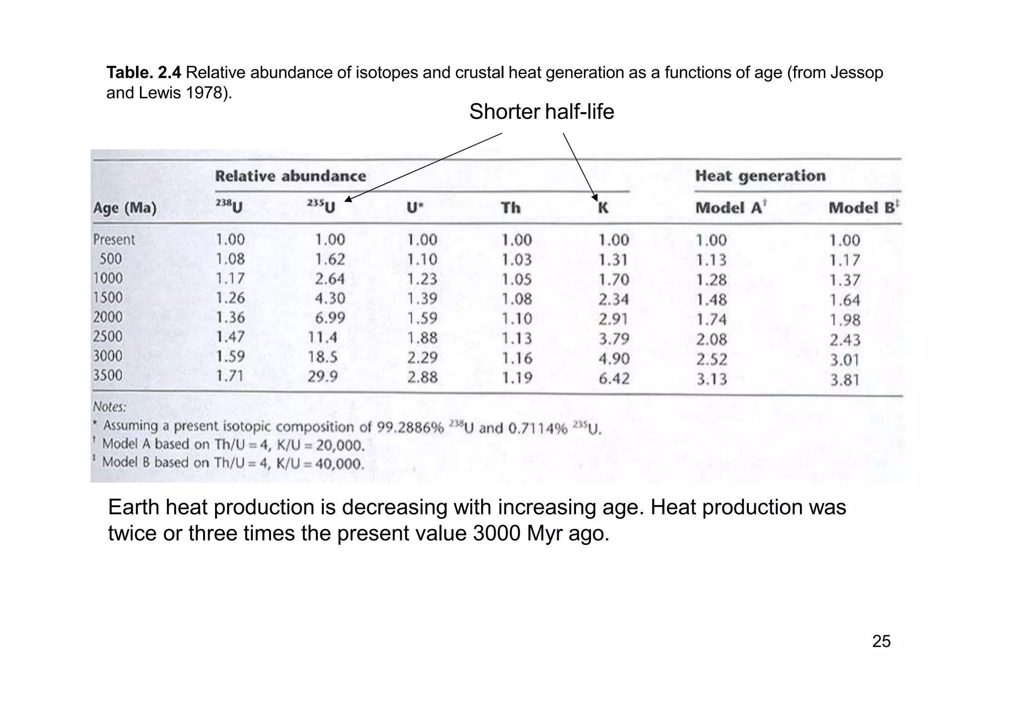
This document discusses the physical state of the lithosphere, including stresses, strains, heat flow, gravity, isostasy, and rock rheology. Specifically, it covers stress and strain in the lithosphere, including lithostatic stress, deviatoric stress, and principal stresses and strains. It also discusses heat flow through conduction and convection, and concepts of isostasy and compensation of topography through density differences. Finally, it examines rock rheology, including fundamentals of rheology, viscosity of the mantle and crust, and elastic versus plastic behavior.


