Machine lectures: Bayes Classifiers

1. Machine Learning
Zahra Sadeghi, PhD
1
Bayesian model

2. Bayes theorem
• Bayes' Theorem, named after 18th-century British
mathematician Thomas Bayes, is a mathematical formula
for determining conditional probability.
• Conditional probability is the likelihood of an outcome
occurring, based on a previous outcome having occurred
in similar circumstances.
• Bayes' theorem provides a way to revise existing
predictions or theories (update probabilities) given new or
additional evidence.
2

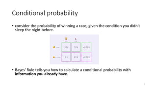
3. Conditional probability
• consider the probability of winning a race, given the condition you didn't
sleep the night before.
• Bayes' Rule tells you how to calculate a conditional probability with
information you already have.
3

4. Bayes Classifier
• Bayesian classifiers are statistical classifiers.
• They can predict class membership probabilities, such as the
probability that a given sample belongs to a particular class.
• Bayesian classifier is based on Bayes’ theorem.
• two important events
• A hypothesis (which can be true or false)
• An evidence (which can be present or absent).
4

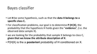
5. • Let H be some hypothesis, such as that the data X belongs to a
specific class C.
• For classification problems, our goal is to determine P (H|X), the
probability that the hypothesis H holds given the ”evidence”, (i.e. the
observed data sample X).
• we are looking for the probability that sample X belongs to class C,
given that we know the attribute description of X.
• P(H|X) is the a posteriori probability of H conditioned on X.
5
Bayes classifier

6. Bayesian classification
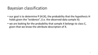
• our goal is to determine P (H|X), the probability that the hypothesis H
holds given the ”evidence”, (i.e. the observed data sample X).
• we are looking for the probability that sample X belongs to class C,
given that we know the attribute description of X.
6

7. Bayes’ theorem
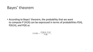
• According to Bayes’ theorem, the probability that we want
to compute P (H|X) can be expressed in terms of probabilities P(H),
P(X|H), and P(X) as
7

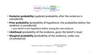
8. • Posterior probability (updated probability after the evidence is
considered)
• Prior probability (probability of hypothesis: the probability before the
evidence is considered)
• your belief in the hypothesis before seeing the new evidence
• Likelihood (probability of the evidence, given the belief is true)
• Marginal probability (probability of the evidence, under any
circumstance)
8

9. Example
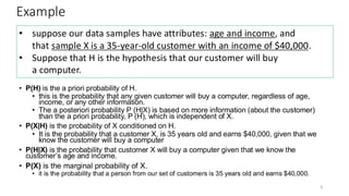
• P(H) is the a priori probability of H.
• this is the probability that any given customer will buy a computer, regardless of age,
income, or any other information.
• The a posteriori probability P (H|X) is based on more information (about the customer)
than the a priori probability, P (H), which is independent of X.
• P(X|H) is the probability of X conditioned on H.
• It is the probability that a customer X, is 35 years old and earns $40,000, given that we
know the customer will buy a computer
• P(H|X) is the probability that customer X will buy a computer given that we know the
customer’s age and income.
• P(X) is the marginal probability of X.
• it is the probability that a person from our set of customers is 35 years old and earns $40,000.
9
• suppose our data samples have attributes: age and income, and
that sample X is a 35-year-old customer with an income of $40,000.
• Suppose that H is the hypothesis that our customer will buy
a computer.

10. Example
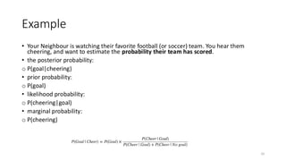
• Your Neighbour is watching their favorite football (or soccer) team. You hear them
cheering, and want to estimate the probability their team has scored.
• the posterior probability:
o P(goal|cheering)
• prior probability:
o P(goal)
• likelihood probability:
o P(cheering|goal)
• marginal probability:
o P(cheering)
10

11. Naive Bayesian Classifier
• Naive Bayesian classifiers assume that the effect of an attribute
value on a given class is independent of the values of the other
attributes.
• This assumption is called class conditional independence.
• It is made to simplify the computation involved and, in this sense,
is considered ”naive”.
11

12. Naive Bayesian Classifier
1. Let T be a training set of samples, each with their class labels.
• There are m classes, C1, C2, . . . , Cm.
• Each sample is represented by an n-dimensional vector, X = {x1, x2, . . . , xn},
depicting n measured values of the n attributes, A1, A2, . . . , An, respectively.
2. Given a sample X, the classifier will predict that X belongs to the class
having the highest a posteriori probability, conditioned on X.
• That is X is predicted to belong to the class Ci if and only if
12

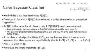
13. • we find the class that maximizes P(Ci|X).
• The class Ci for which P(Ci|X) is maximized is called the maximum posteriori
hypothesis.
• As P(X) is the same for all classes, only P(X|Ci)P(Ci) need be maximized.
• In order to predict the class label of X, P(X|Ci)P(Ci) is evaluated for each class Ci .
• The classifier predicts that the class label of X is Ci if and only if it is the class that maximizes
P(X|C i)P(Ci).
• If the class a priori probabilities, P(Ci), are not known, then it is commonly
assumed that the classes are equally likely, that is, P(C1) = P (C2) = . . . = P (Cm)
• P(Ci) = freq(Ci,T )/|T|.
• we would therefore maximize P(X|Ci).
13
Naive Bayesian Classifier

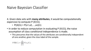
14. 4. Given data sets with many attributes, it would be computationally
expensive to compute P (X|Ci).
• P(X|Ci) = P(x1,x2,…,xn|Ci)
• In order to reduce computation in evaluating P (X|Ci), the naive
assumption of class conditional independence is made.
• This presumes that the values of the attributes are conditionally independent
of one another, given the class label of the sample.
14
Naive Bayesian Classifier

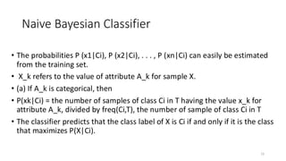
15. • The probabilities P (x1|Ci), P (x2|Ci), . . . , P (xn|Ci) can easily be estimated
from the training set.
• X_k refers to the value of attribute A_k for sample X.
• (a) If A_k is categorical, then
• P(xk|Ci) = the number of samples of class Ci in T having the value x_k for
attribute A_k, divided by freq(Ci,T), the number of sample of class Ci in T
• The classifier predicts that the class label of X is Ci if and only if it is the class
that maximizes P(X|Ci).
15
Naive Bayesian Classifier

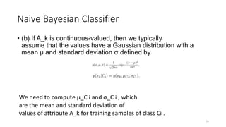
16. • (b) If A_k is continuous-valued, then we typically
assume that the values have a Gaussian distribution with a
mean µ and standard deviation σ defined by
16
Naive Bayesian Classifier
We need to compute µ_C i and σ_C i , which
are the mean and standard deviation of
values of attribute A_k for training samples of class Ci .

17. Bayes decision theory
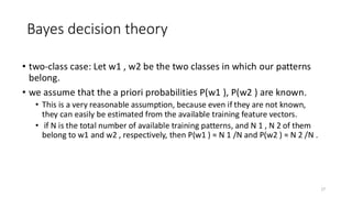
• two-class case: Let w1 , w2 be the two classes in which our patterns
belong.
• we assume that the a priori probabilities P(w1 ), P(w2 ) are known.
• This is a very reasonable assumption, because even if they are not known,
they can easily be estimated from the available training feature vectors.
• if N is the total number of available training patterns, and N 1 , N 2 of them
belong to w1 and w2 , respectively, then P(w1 ) ≈ N 1 /N and P(w2 ) ≈ N 2 /N .
17

18. Bayes decision theory
18
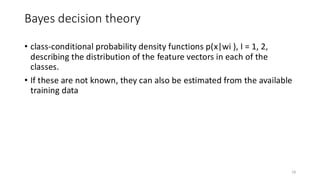
• class-conditional probability density functions p(x|wi ), I = 1, 2,
describing the distribution of the feature vectors in each of the
classes.
• If these are not known, they can also be estimated from the available
training data

19. Bayes decision theory
19
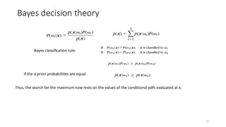
Bayes classification rule:
if the a priori probabilities are equal
Thus, the search for the maximum now rests on the values of the conditional pdfs evaluated at x.

20. Bayes decision theory
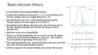
• an example of two equiprobable classes
• shows the variations of p(x|wi ), i = 1, 2, as functions of x
for the simple case of a single feature (l = 1).
• The dotted line at x 0 is a threshold partitioning the
feature space into two regions, R 1 and R 2 .
• According to the Bayes decision rule, for all values of x in
R1 the classifier decides w1 and for all values in R2 it
decides w2 .
• decision errors are unavoidable
• There is a finite probability for an x to lie in the R2 region
and at the same time to belong in class w1 . The same is
true for points originating from class w2 .
• The total probability, Pe , of committing a decision error for
the case of two equiprobable classes
• which is equal to the total shaded area under the curves
20

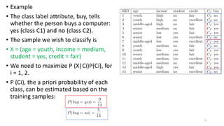
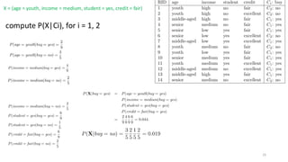
21. • Example
• The class label attribute, buy, tells
whether the person buys a computer:
yes (class C1) and no (class C2).
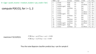
• The sample we wish to classify is
• X = (age = youth, income = medium,
student = yes, credit = fair)
• We need to maximize P (X|Ci)P(Ci), for
i = 1, 2.
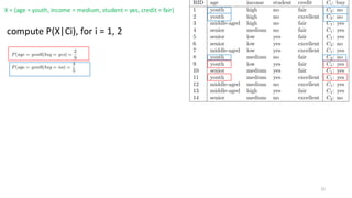
• P (Ci), the a priori probability of each
class, can be estimated based on the
training samples:
21

22. compute P(X|Ci), for i = 1, 2
X = (age = youth, income = medium, student = yes, credit = fair)
22

23. compute P(X|Ci), for i = 1, 2
X = (age = youth, income = medium, student = yes, credit = fair)
23

24. compute P(X|Ci), for i = 1, 2
X = (age = youth, income = medium, student = yes, credit = fair)
24
Exercise:

25. compute P(X|Ci), for i = 1, 2
X = (age = youth, income = medium, student = yes, credit = fair)
25

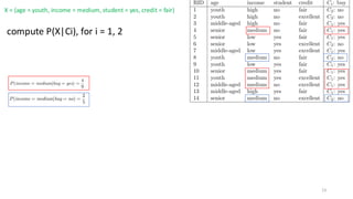
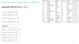
26. compute P(X|Ci), for i = 1, 2
maximizes P (X|Ci)P(Ci):
Thus the naive Bayesian classifier predicts buy = yes for sample X
X = (age = youth, income = medium, student = yes, credit = fair)
26

27. Minimizing the Average Risk
• The classification error probability is not always the best criterion to be adopted
for minimization.
• This is because it assigns the same importance to all errors.
• However, there are cases in which some wrong decisions may have more serious
implications than others.
• For example, it is much more serious for a doctor to make a wrong decision and a
malignant tumor to be diagnosed as a benign one, than the other way round.
• If a benign tumor is diagnosed as a malignant one, the wrong decision will be
cleared out during subsequent clinical examinations.
• However, the results from the wrong decision concerning a malignant tumor may
be fatal.
• Thus, in such cases it is more appropriate to assign a penalty term to weigh each
error.
27

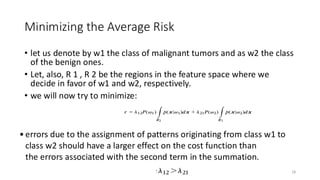
28. Minimizing the Average Risk
• let us denote by w1 the class of malignant tumors and as w2 the class
of the benign ones.
• Let, also, R 1 , R 2 be the regions in the feature space where we
decide in favor of w1 and w2, respectively.
• we will now try to minimize:
28
• errors due to the assignment of patterns originating from class w1 to
class w2 should have a larger effect on the cost function than
the errors associated with the second term in the summation.​

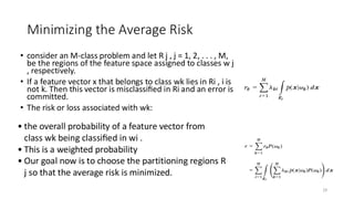
29. • consider an M-class problem and let R j , j = 1, 2, . . . , M,
be the regions of the feature space assigned to classes w j
, respectively.
• If a feature vector x that belongs to class wk lies in Ri , i is
not k. Then this vector is misclassified in Ri and an error is
committed.
• The risk or loss associated with wk:
29
Minimizing the Average Risk
• the overall probability of a feature vector from
class wk being classified in wi .​
• This is a weighted probability​
• Our goal now is to choose the partitioning regions R
j so that the average risk is minimized.