This document presents a new method for locating ungrounded faults in underground distribution systems using wavelet analysis and artificial neural networks (ANNs). Voltage and current signals are simulated for different fault types, locations, and conditions using EMTP software. Wavelet analysis is used to extract features from the signals related to fault classification and location. ANNs are then applied to classify fault types based on the extracted features and to determine the fault location for each fault type based on additional extracted features. The results indicate the technique can accurately locate faults under a variety of system conditions.

1. Abstract
This paper presents the results of investigations into a new
fault location technique based on a new modified cable model,
in the EMTP software. The simulated data is then analysed
using advanced signal processing technique based on wavelet
analysis to extract useful information from signals and this is
then applied to the artificial neural networks (ANNs) for
locating ungrounded shunt faults in a practical underground
distribution system. The paper concludes by comprehensively
evaluation the performance of the technique developed in the
case of ungrounded short circuit faults. The results indicate that
the fault location technique has an acceptable accuracy under a
whole variety of different systems and fault conditions.
Keywords: Fault location, ungrounded faults, underground
distribution cable, wavelet, neural network
1. Introduction
In recent years, there have been many activities in using
fault generated travelling wave methods for fault location and
protection. The travelling wave current-based fault location
scheme in which the distance to fault is determined by the
time differences measured at the sending end between an
incident wave and the corresponding wave reflected from the
fault have been developed for permanent faults in underground
low voltage distribution networks by S. Navaneethan et. al. in
ref. [1]. However, due to the limitation of the bandwidth of the
conventional CT (up to a few GHz) and VT (up to 50 kHz),
the accuracy of fault location provided by such a scheme is not
satisfactory for a power cable. Also there have been many
activities in using power frequency (low frequency) for fault
location and protection. Aggarwal et. al. in ref. [2] present a
new technique in single-ended fault locationfor overhead
distribution systems, which is based on the concept of
superimposed components of voltages and currents rather than
total quantities and also special filtering techniques have been
utilised to accurately extract the fundamental phasors from the
measured fault signals. However, in such techniques which are
based on power frequency signals, some useful information
associated with high frequencies in transient condition is
missed.
This paper presents a new off-line method in cable
ungrounded fault location based on signal processing using
wavelet and ANNs. A practical 11 kV underground power
distribution system (DS) with remote source is simulated using
the EMTP software; the faulted current and voltage responses
are then extracted from the sending end for different faults and
fault conditions. The effect of transducers (CTs and VTs) and
hardware errors such as anti-aliasing filters and quantisation
are taken into account; the information processed throughout
the fault locator algorithm is thus very close to real-life
situation. Finally, the simulated data is processed in order to
locate the fault point.
2. Data simulation
In order to obtain the voltage and the current signals under
different faults and conditions, a practical three-phase
underground distribution network shown in Fig. 1 has been
considered.
Fig. 1. Practical 3-phase underground distribution network
The specifications of the various elements in Fig (1) are as
follows:
Source: VL = 11kV, f=50Hz, Xs:Rs=10, Xs=2Ω, Rs=0.2Ω
Cables: XLPE, Three-phase pipe type cable (core + grounded
sheath)
Transformer: S=1 MVA
Winding 1 : VL=11kV, Rp=1 Ω, Lp=28.6mH
Winding 2 : VL=380V, Rs=0.00044 Ω, Ls=0.0114mH
Load 1: Three-phase static Load: VL=380 Vrms, f=50 Hz,
PL=92.62kW, QL=69.252kVAR
Load 2: The combination of a three=phase static and dynamic
loads
Dynamic Load: VL=380 Vrms, f=50 Hz, P=200 HP,
Static Load: PL=92.62kW, QL=69.252kVAR, VL=380
Vrms
Load 3: Three-phase static Load: VL=11 kVrms, f=50 Hz,
PL=124kW, QL=952kVAR
In this paper, the simulation of the quantization process is
based on 16-bit A/D converter with ±10V by using MATLAB
program. In order to keep the voltage and current signals in
range ±10V, these signals are divided by 2200 and 700
respectively, which are 1/10 of maximum amount of voltage
and current signals under all conditions.
A NEW APPROACH TO UNGROUNDED FAULT LOCATION IN A
THREE-PHASE UNDERGROUND DISTRIBUTION SYSTEM USING
COMBINED NEURAL NETWORKS & WAVELET ANALYSIS
Jamal Moshtagh R. K. Aggarwal
University of Bath, UK University of Bath, UK
moshtagh79@yahoo.com r.k.aggarwal@bath.ac.uk
1-4244-0038-4 2006
IEEE CCECE/CCGEI, Ottawa, May 2006
376
Authorized licensed use limited to: BROWN UNIVERSITY. Downloaded on April 8, 2009 at 15:51 from IEEE Xplore. Restrictions apply.

2. It is apparent that both the steady and transient states of the
voltage and current signals can be affected by some important
parameters such as the type of fault, inception angle and
distance to fault for ungrounded fault type. In order to obtain
useful information from signals in the signal processing stage
and mapping the extracted information to the location of fault
in artificial intelligent (AI) stage, it is necessary to obtain
voltage and current signals, different fault types and different
conditions in the data simulation stage. In this respect, two
types of fault including phase to phase short-circuit fault (3
cases ab-sc, ac-sc and bc-sc) and three-phase short-circuit
fault(one case abc-sc) also three inception angles (including
90, 135 and 180 degrees) and 13 distances of fault from
recording point (including 50m, 100m, 500m, 900m, 1100m,
1500m, 1900m, 2100m, 2500m, 2900m, 3100m, 3500m and
3900m) are simulated.
Figs(2 to 3) typifies the three-phase voltages and three-
phase currents, respectively. Each figure contains two graphs
associated with two different inception angles 90 and 180
degrees for the condition of 1100m distance in the case of bc-
sc fault. Fig(2) depicts the voltage signals and as can be seen,
initial distortions are much higher in the case of inception
angle 180 degrees because of the maximum step change in
phase voltage associated with this fault. Also the amplitude of
voltage in both faulted phases b and c considerably fall after
occurring the fault.
Fig(3) shows the current signals and the magnitude of
current in faulted phases increase significantly. In the case of
90 degree fault (i.e. a fault near zero phase voltage), there is a
large DC offset in the current signals and little distortion in the
voltage signals.
Figs(4 & 5) show the three phase voltage and current
waveforms for a 3-phase fault (abc-sc), fault locations=
1100m, 2100 and 3100m and without remote source
connected. Fig(4) depicts voltage signals and as it can be seen
that the initial distortions are much higher and the transients
die down much slower in the case of the closer fault. Also,
Fig(5) shows the current signals and it is clearly evident that
the currents in three faulted phases increase after fault and as
expected are much smaller in the case of location at 3100m.
Fig. 2. Three phases of voltage signals, bc-sc fault, L=1100m
. Fig. 3. Three phases of current signals, bc-sc fault, L=1100m
Fig. 4. Voltage signals, abc-sc, inception angle.=135degrees
Fig. 5. Current signals, abc-sc, inception angle.=135degrees
3. Feature Extraction Using Wavelet
Transient signal analysis has been extensively used in fault
location and condition monitoring of power system lines and
cables. The time and frequency information can be calculated
using techniques such as Fast Fourier Transform (FFT), Short-
377
Authorized licensed use limited to: BROWN UNIVERSITY. Downloaded on April 8, 2009 at 15:51 from IEEE Xplore. Restrictions apply.

3. Time Fourier Transform (STFT) and Wavelet Transform
(WT). FFT and STFT techniques yield good information on
the frequency content of the transient, but the time at which a
particular disturbance in the signal occurred is lost.
In this paper, a new approach based on feature extraction
using the WT is presented. WT possesses some unique
features that make it very suitable for this particular
application. It maps a given function from the time domain
into time-scale domain. Unlike the basis function used in
Fourier analysis, the wavelets are not only localized in
frequency but also in time. This localization allows the
detection of the time of occurrence of abrupt disturbances,
such as fault transients.
3.1. Wavelet Transform
In the case of WT, the analysing function, which is called
wavelets, will adjust their time-widths to their frequency in
such a way that higher frequency wavelets will be very narrow
and lower frequency ones will be broader. This property of
multi-resolution is particularly useful for analysing fault
transients which localize high frequency components
superposed on power frequency signals (Manago & Abur [3]).
WT of sampled waveforms can be obtained by
implementing the discrete WT which is given by:
∑
−
=
k
m
m
m a
kan
hkf
a
nmfDWT )()(
1
),,(
0
0*
0
(1)
where, the parameters
m
a0 and k
m
a0 are the scaling and
translation constant respectively, k and m being integer
variables and h is the wavelet function which may not be real,
as assumed in the above equation for simplicity. In a standard
discrete WT (DWT), the coefficients are sampled from the
continuous WT on a dyadic grid, a0=2, yielding
2/1,.1 1
0
0
0 == −
aa , etc. Actual implementation of the (DWT)
involves successive pairs of high-pass and low-pass filters at
each scaling stage of the WT. At each detail, there is a signal
appearing at the filter output at the same sample rate as the
input; thus, by using a sample rate F and scaling by two
(a0=2), Eq.(2) shows the association of each scale 2m
with a
frequency band containing distinct components of signals.
Frequency band of scale 2m
=F/2m+2
→F/2m+1
(2)
In this paper the original signals have been sampled at 100
kHz and passed through a DWT; thus according to Eq. (2) the
frequency band for detailed and approximate signals are;
25kHz to 50kHz at detail-1, 12.5kHz t0 25kFz at detail-2, etc.
3.2. Choice of Mother Wavelet
Choosing of mother wavelets plays an important role in
localizing and depends on a particular application.
Researchers, in the study of underground power distribution
transients are particularly interested in detecting and analysing
short duration, fast decaying and oscillating type of high and
low frequency voltage and current signals. One of the most
popular mother wavelets suitable for a wide range of
applications used is Daubichies’s wavelet. In this respect, db4
wavelet with 5 level of decomposing of signals has been
considered herein.
3.3. Feature Extraction in Fault Classification
The process comprises two stages including; 1- fault
classification 2- fault location. At first, the original signals are
passed through a DWT then 5-detailed and one approximate
signals are extracted. With regard to statistics option in
wavelet and data processing on approximate signals of the
voltage and current phases, it was observed that some useful
information can be extracted from standard deviation (SD) of
approximate-5 signals in fault classification, since the amount
of SD for every input data with dimension 6 (three voltage
phases and three current phases) has an obvious relationship
with the type of fault and faulted phases.
Figs (6 & 7) show such data which is used in the fault
classification associated with the type of fault and faulted
phases. Each figure comprises two graphs associated with
voltage phases and current phases. Each graph shows three
waveforms related to the three phases and each waveform
depicts the SD of approximate-5 of signal for the all
conditions dealt with in the previous section. Also, each
waveform contains 3 separate the parts. Each part corresponds
to the 13 locations and the same inception angle. As it can be
seen, there is a significant difference between the faulted
phases and healthy phase.
Fig. 6. SD of approximate-5 signal in the case of bc-sc fault
Fig. 7. SD of approximate-5 signal in the case of abc-sc fault
378
Authorized licensed use limited to: BROWN UNIVERSITY. Downloaded on April 8, 2009 at 15:51 from IEEE Xplore. Restrictions apply.

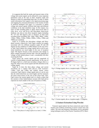
4. 3.4. Feature Extraction in Fault Location
In order to locate an ungrounded fault, three important
parameters are employed; 1- ratio of peak-peak voltage
approximate to peak-peak current approximate at level five
(a_ppv/a_ppi), 2- sine of phase-shift between current and
voltage approximate at level 5 multiple by a_ppv/a_ppi,
(sin(φi-φv).v/i), 3- ratio of SD of voltage approximate to SD
of current approximate at level 5 (SDv/SDi). It should be
mentioned that these three parameters are employed only for
the faulted phases in the case of a phase to phase fault, but
only phase-a is considered in the case of three-phase short
circuit fault. In order to obtain more accurate results, the
signals are normalized according to Eq. (3).
)/()( minmaxmin IIIIInormed −−= (3)
Figs. (8 & 9) show the results for 39 fault conditions,
associated with three-phase and phase-b to phase-c faults. As
can be seen, Fig. (8) comprises 3 graphs and Fig. (9) also
contains 3 graphs correspond to the phase-b and here, because
of similarity the graphs related to phase-c have not been
considered. Each graph consists of three parts relating to three
inception angles and each part corresponds to the 13 fault
locations, all of which are ascending by virtue of an increase
in the distance to fault location; as it can be seen, there is an
apparent relationship between considered parameters and fault
location for both types of fault.
Fig. 8. Three parameters used in fault location, abc-sc fault
Fig. 9. Six parameters used in fault location, bc-sc fault g
4- Fault Location Based on ANNs
ANNs have emerged as a powerful pattern recognition
technique and act on data by detecting some form of
underlying organisation not explicitly given or even known by
human experts and it possesses certain features which are not
attainable by the conventional methods. In this respect, this
paper describes a new method for accurate fault location based
on the ANNs technique. The successful development of ANNs
approaches depends on the successful learning of the correct
relationship or mapping between the input and output patterns
by the ANNs [4]. In order to achieve this, practical issues
surrounding the design, training and testing of an ANN such
as the best network size, generalization versus memorisation,
feature extraction, convergence of training process and scaling
of signals have been addressed and examined.
In order to find the best topology for accurate fault location,
an extensive series of studies have revealed that it is not
satisfactory to merely employ a single ANN and attempt to
train it with a large amount of data. A much better approach is
to separate the problem into two parts: firstly to employ and
train an ANN to classify the faults; secondly, to use separately
ANNs (one for each type of fault and faulted phases) to
accurately locate the actual fault position. Fig. (10) shows the
fault location scheme based on ANNs.
Fig. 10. Schematic diagram of fault location technique
There are many types of ANNs but the most commonly used
are the multi-layer feed-forward networks, as, a three-layer
network (input, one hidden and output layers). Because of this,
a fully connected three-layer feed-forward ANNs with
Levenberg-Marquardt (LM) learning algorithm has been used
in the complete fault classification and fault location networks.
Tabel-1 depicts the specifications of employed ANNs in
proposed fault location technique.
Table 1. Specifications of employed ANNs
NN N1 N2 N3 N4 f1(x) f2(x)
NNtf 156 6 4 3 TanSig Linear
NNab 39 6 4 1 TanSig TanSig
NNac 39 6 4 1 TanSig TanSig
NNbc 39 6 4 1 TanSig TanSig
NNabc 39 3 7 1 TanSig TanSig
Where N1=number of training data, N2=dimension of input
layer, N3=number of neuron in hidden layer, N4=number of
neuron in output layer, f1(x)=transfer function in hidden layer
and f2(x)=transfer function in output layer.
379
Authorized licensed use limited to: BROWN UNIVERSITY. Downloaded on April 8, 2009 at 15:51 from IEEE Xplore. Restrictions apply.

5. The NNtf recognizes the type of fault and faulted phases for
ungrounded faults. The output of the NNtf comprises 3
variables A, B and C; of these, a value close to unity for any of
the variables corresponds to the appropriate a, b or c phases
being faulted. The NNab-sc, NNac-sc, NNbc-sc and NNabc-sc
architectures are shown in Table-1 and determine the location
of fault in the case of phase to phase and three-phase short
circuit fault.
5. Analysis of Test Results
In order to analyse the accuracy of the proposed method,
seven groups of data test have been selected which are
different and unseen from that used for training. Then,
sensitivity of method to the system parameters such as
inception angle, system elements (load taps, the length of
cable, remote source) and to the external faults is evaluated.
These seven groups of data test are as follows:
Group 1: This group contains such data which are obtained
from normal system shown in fig (1) without remote source.
18 data are employed based on two types of fault (bc-sc &
abc-sc) and 9 conditions for each fault. Table-2 depicts 9
locations, not used during training, with different inception
angles.
Group 2: This group is similar to group 1 but with remote
source.
Group 3: This group of data is associated with changing the
location of the second load (shown in fig (1)) from 2000m to
1500m. 14 data test sets are used based on two faults and 7
conditions for each fault. Table-2 shows seven locations with
different inception angles.
Group 4: In this group, data are obtained from DS shown in
fig (1) based on changing the amount of three employed loads
to double. This group also contains 14 data similar to group 3.
Group 5: This group contains such data which is based on
doubling the amount of loads and replacing the loads 1 & 2
shown in fig (1). 14 data are obtained based on the same
condition in group 3 & 4.
Group 6: This group comprises 14 data test based on the
same condition shown in Table-2 and the same network shown
in fig (1), but the length of cable in each section is changed
from 1000m to 1500m.
Group 7: This group contains 2 data based on two faults as
external fault (fault occurs before the measurement point).
Table 2. Group-1 of data test
Groups 1 & 2 Groups 3,4,5 &6
Location Θ (Deg.) Location Θ (Deg.)
80 m 117 80m 117
350 m 117 350m 117
750 m 117 1100m 90
1250 m 162 1750m 162
1750 m 162 2500m 135
2250 m 162 3250m 117
2750 m 162 3800m 117
3250 m 117
3800 m 117
5.1. Performance of Fault Classification
In order to quantitatively evaluate the performance of the
fault classification technique, the NNtf was tested by seven
aforementioned data test groups including over 92 system and
fault conditions. It is evident from the results that except
group-7 of data test (external fault) the number of error
decision was zero in relation to the NNtf; therefore it can be
concluded that this method is indead to classify the type of
fault and recognizes the faulted phases.
5.2. Performance of Fault Location
The trained ANNs involved in the second stage of the fault
location technique were tested by seven aforementioned
groups of data test. The error for fault location is expressed as
a percentage of the length of the cable, and is given as:
100
)_(
)_()_(
% ×
−
=
lengthcable
locationdesiredlocationactual
error (4)
5.2.1. Effect of fault parameters. The inception angle
significantly affects the fault transient voltage and current
signals and it is vitally important to verify the effect of this
parameter on the performance of the proposed technique.
Table-3 show the accuracies attained for group-1&2 of test
results. It is clearly evident from the results that the ANNs
give very accurate evaluation of fault position and the
maximum and mean of error correspond to the bc-sc and the
abc-sc faults are (0.275 & 0.07) and (0.85 & 0.367) percent
respectively. This study clearly demonstrates that the
algorithm is virtually immune to any errors caused by either
the higher frequency transients, which are associated with
faults near voltage maximum or DC offset caused by faults
near voltage zero. This feature is important since in practice,
faults can occur at any point on wave i.e. the fault inception
angle cannot be defined in advance.
5.2.2. Effect of remote source. It is well known that a remote
infeed can adversely affect the accuracy of conventional fault
locators. In this respect, the algorithm was tested based on
group-2 of data test. Table-3 depicts the results. In comparison
to the previous case associated without remote source, it is
evident that the presence of a remote source has only a slight
effect on accuracy particularly in the case of phase to phase
fault, as the maximum and the mean of error associated with
two faults increased very slightly to (1.957 & 0.586) and
(0.735 & 0.408) respectively. These small changes can be
directly attributed to the fact that with a remote source, the
current changes in the healthy phase in terms of magnitude
and distortion.
5.2.3. Effect of load taps. It is apparent that load taps
significantly affect the fault transient waveforms. Therefore, it
is vitally important to verify the effect of the load taps on the
performance of the proposed technique. In this respect three
groups-3,4&5 are considered and Table-4&5 depict the
results. It is clearly evident from the results that the accuracy
achieved in fault location is very high; being less than 1%
380
Authorized licensed use limited to: BROWN UNIVERSITY. Downloaded on April 8, 2009 at 15:51 from IEEE Xplore. Restrictions apply.

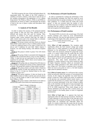
6. error in all the test cases. Thus it can be concluded that the
ANNs give accurate evaluation that is largely independent on
the load taps. This is a significant advantage since being
different load taps at different location of DS is inevitable.
5.2.4. Effect of cable length. The cable length can vary
considerably in the DS, it is vitally important to ascertain as to
what extent the fault location accuracy is affected as a result of
a change in the cable length. Table-5 illustrates the
performance of the ANN-based technique when subjected to
the cable length 1500m instead of 1000m for each section of
such system shown in fig.(1) (group-6 of the data test). The
results clearly demonstrate that the accuracy achieved in fault
location is very high; being less than 0.85% error in all the test
cases and shows that the ANNs give accurate evaluation of
fault position that is largely independent on the cable length. D
is real distance and L is obtained location by technique.
Table 3. Performance of fault location based on group-1&2 of data test
bc-sc, G1 abc-sc, G1 bc-sc, G2 abc-sc, G2D
(m) L
(m)
%e L
(m)
%e L (m) %e L (m) %e
80 79.7 .01 72.4 .19 72.5 .19 72.7 .18
350 350 .00 350 .00 339 .27 349.9 .00
750 749 .02 759 .23 738 .31 759 .21
1250 1253 .07 1263 .32 1245 .12 1266 .40
1750 1751 .02 1764 .35 1754 .12 1768 .47
2250 2252 .05 2261 .27 2273 .58 2268 .45
2750 2753 .07 2766 .4 2805 1.4 2772 .57
3250 3246 .1 3284 .85 3328 1.9 3279 .73
3800 3811 .27 3827 .67 3814 .36 3825 .64
M.
E%
0.07 0.367 0.586 0.408
Table 4. Performance of fault location based on group-3&4 of data test
bc-sc, G3 abc-sc, G3 bc-sc, G4 abc-sc,G4D
(m) L
(m)
%e L
(m)
%e L
(m)
%e L
(m)
%e
80 79.8 .00 72.4 .19 75.6 .08 72.0 .2
350 350 0.0 350 .00 356.4 .16 350.3 .01
1100 1100 0.0 1103 .08 1098 .05 1097 .08
1750 1752 .05 1765 .37 1750 .0 1757 .18
2500 2499 .02 2505 .13 2502 .05 2496 .1
3250 3242 .2 3289 .98 3243 .17 3273 .57
3800 3808 .2 3825 .62 3772 .7 3815 .37
M.
E%
0.068 0.337 0.174 0.19
Table 5. Performance of fault location based on group-5&6 of data test
bc-sc, G5 abc-sc, G5 bc-sc, G6 abc-sc, G6D
(m) L
(m)
%e L
(m)
%e L
(m)
%e L
(m)
%e
80 75.6 .11 72.0 .2 80.2 .00 72.4 .19
350 346.3 .09 350.3 .01 350.5 .01 350.1 .00
1100 1099 .02 1100 .0 1100 .0 1103 .07
1750 1757 .17 1760 .25 1754 .1 1766 .4
2500 2507 .17 2492 .2 2503 .07 2501 .02
3250 3246 .1 3263 .32 3253 .07 3281 .77
3800 3770 .75 3809 .22 3823 .57 3834 .85
M.
E%
0.204 0.172 0.12 0.331
5.2.5. Effect of External Faults. In any fault location
technique, although a high accuracy for internal faults is of
primary concern, nonetheless, it should also be stable under
external faults. For the fault location technique described
herein, an external fault produces an estimation which is
consistently very much and negative distance. It is evident
from the results that when the ANNs give such abnormally
high and negative values, then it can be safely assumed that
the fault is external.
6. Conclusion
In this paper at first, a new method to analyse power
distribution system transient signals based-EMTP is proposed
by using WT technique. This method offers important
advantages over other methods such as FFT and STFT due to
good time and frequency localisation characteristics. Analysis
results presented clearly show that particular wavelet
components can be used as the features to locate the fault in
underground DS. Then an accurate fault location technique
based on ANN is developed, as an ANN is trained to classify
the fault type and separate ANNs are designed to accurately
locate the actual ungrounded fault position on a practical
underground DS. In this respect, three-layer feed-forward
ANNs and the LM algorithm is used to adopt the weights and
biases to achieve the desired non-linear mapping from inputs
to outputs. Through a series of tests and modifications, it is
shown that the ANNs can very accurately classify the type of
fault under different system and fault conditions. In order to
illustrate the effectiveness of fault location based-ANNs
technique, each ANN is tested with a separate set of unseen
data and their performance on the accuracy of the results are
presented. The results presented herein, clearly show that the
proposed method gives a high accuracy in fault location under
a whole variety of different system and fault conditions.
Thus it can be concluded that the proposed approach based
on combined WT and ANN is robust to different case studies;
this is a significant advantage and can be directly attributed to
the fact that WT technique effectively extracts the very crucial
time-frequency features from DS transient signals and ANN
approach is able to give a very high accuracy in the fault
classification and fault location.
References
[1] S Navaneethan, J Soraghan, W H Siew, F Mcpherson & P F Gale,
“Automatic Fault Location for Underground Low Voltage
Distribution Networks”, IEEE Transactions on Power Delivery,
Vol. 16, No. 2, pp. 346-351, April 2001.
[2] R.K.Aggarwal, Y.Aslan, A.T.Johns, “New concept in fault
location for overhead distribution systems using superimposed
components”, IEE Journal, Vol. 146, pp. 209-216, May 1999
[3] F H Magnago, and A Abur, 1998 IEEE, “Fault location using
wavelets”, Vol.13, No.4, 1475-1480
[4] Stamatios V Kartalopoulos, “Understanding Neural Network and
Fuzzy Logic: Basic Concepts and Applications”, The Institute of
Electrical and Electronics Engineers, Inc., New York, 1996.
381
Authorized licensed use limited to: BROWN UNIVERSITY. Downloaded on April 8, 2009 at 15:51 from IEEE Xplore. Restrictions apply.