2-Two-wire lines theory - Part A, de la teoria de trasmision de dos lineas.pdf
1.
Two wire-line theory
PartA
Taken from LÍNEAS DE TRANSMISIÓN by Rodolfo Neri Vela
Translated and prepared and by: Eng . Luis Carlos Gil Bernal MsC Telematics
2.
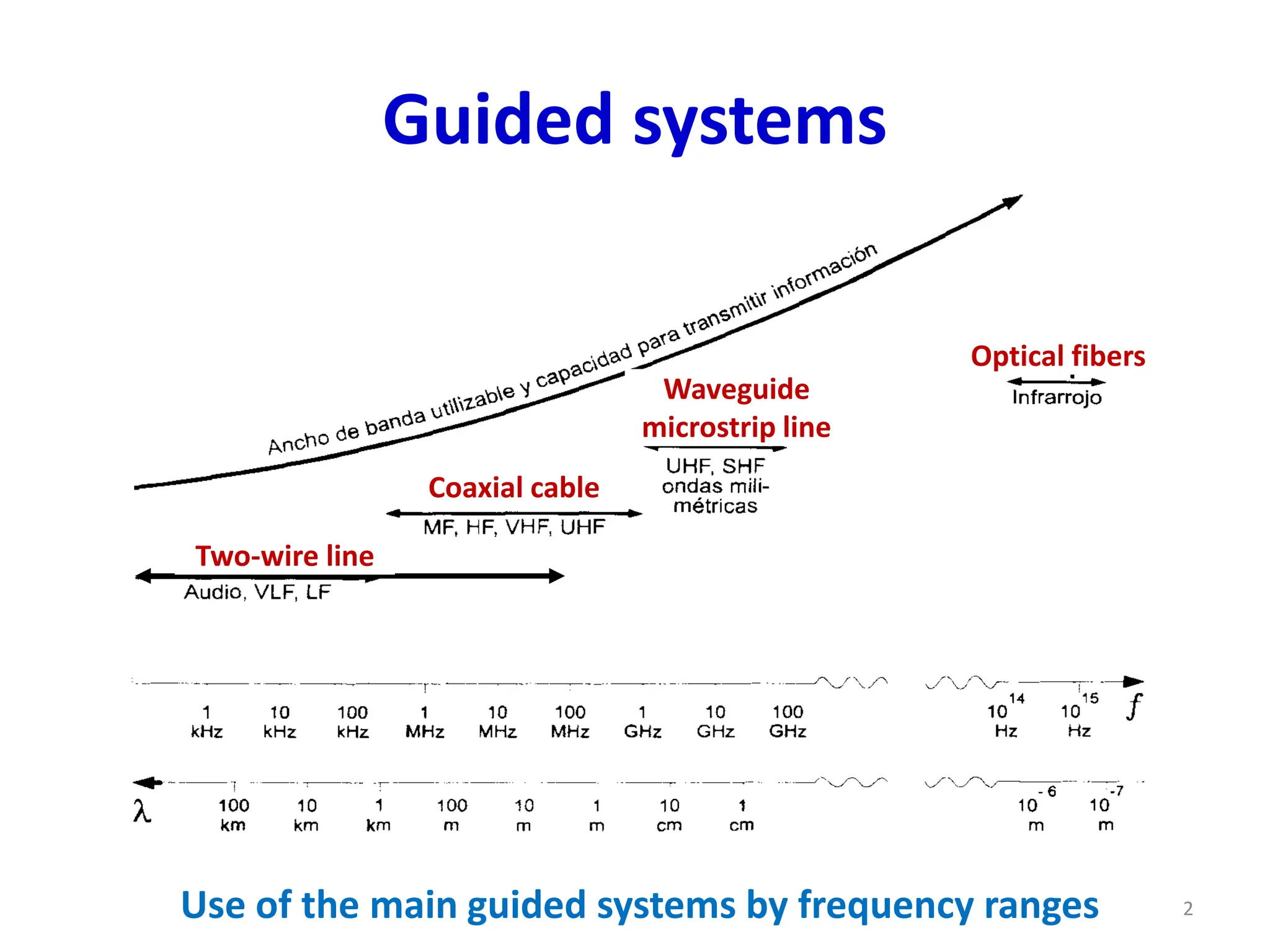
Guided systems
Use ofthe main guided systems by frequency ranges 2
Two-wire line
Coaxial cable
Waveguide
microstrip line
Optical fibers
3.
Two-wire lines theory
•One of the means of transmitting
power or information is by guided
structures.
• Guided structures serve to guide (or
direct) the propagation of energy
from the source to the load.
3
4.
Two-wire lines theory
•Typical examples of such structures
are:
–Transmission lines,
–Waveguides and,
–Fiber optics.
• First, we will consider transmission
lines.
4
5.
Two-wire lines theory
•Transmission lines are commonly
used in:
–power distribution (at low
frequencies) and,
–in communications (at high
frequencies).
5
6.
Two-wire lines theory
•Various kinds of transmission lines
such as the twisted-pair and coaxial
cables (thin-net and thick-net) are
used:
–In telephony,
–in TV cable networks and,
–in computer networks.
6
7.
Two-wire lines theory
•The source may be a hydroelectric
generator, a transmitter, or an
oscillator.
• The load may be a factory, an
antenna, or an oscilloscope,
respectively.
7
8.
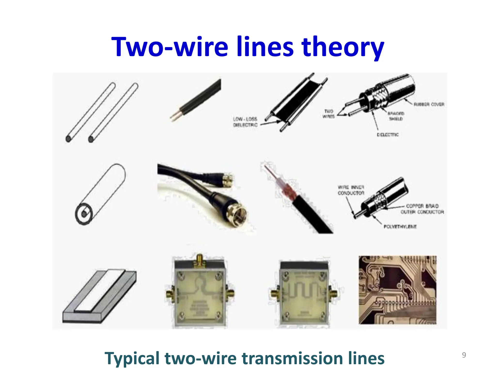
Two-wire lines theory
•Typical transmission lines include
coaxial cable, a two-wire line, a
parallel-plate or planar line, a wire
above the conducting plane, and a
microstrip line.
• Each of these lines consists of two
conductors in parallel.
8
Two-wire lines theory
•Coaxial cables are routinely used in
electrical laboratories and in
connecting TV sets to TV antennas.
Microstrip lines are particularly
important in integrated circuits
10
11.
General concepts
• Linesthat transmit information in
Traverse Electromagnetic (TEM)
propagation mode, such as two-wire
line and coaxial, or essentially TEM,
such as microstrip, can be analyzed:
–Directly solving Maxwell's
equations (EM field theory)
–Using general circuit theory.
11
12.
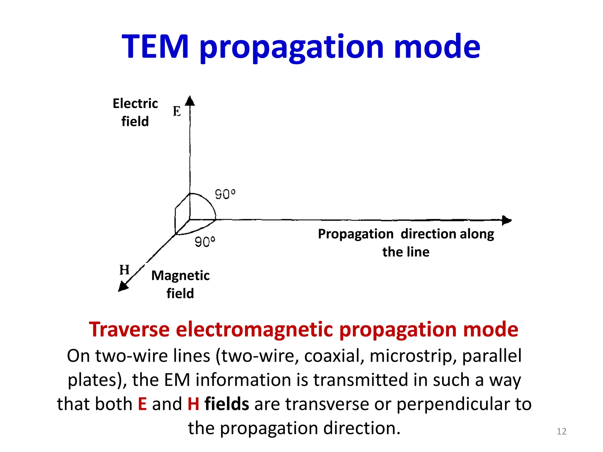
TEM propagation mode
Traverseelectromagnetic propagation mode
On two-wire lines (two-wire, coaxial, microstrip, parallel
plates), the EM information is transmitted in such a way
that both E and H fields are transverse or perpendicular to
the propagation direction.
Campo
eléctrico
Campo
magnético
12
Electric
field
Magnetic
field
Propagation direction along
the line
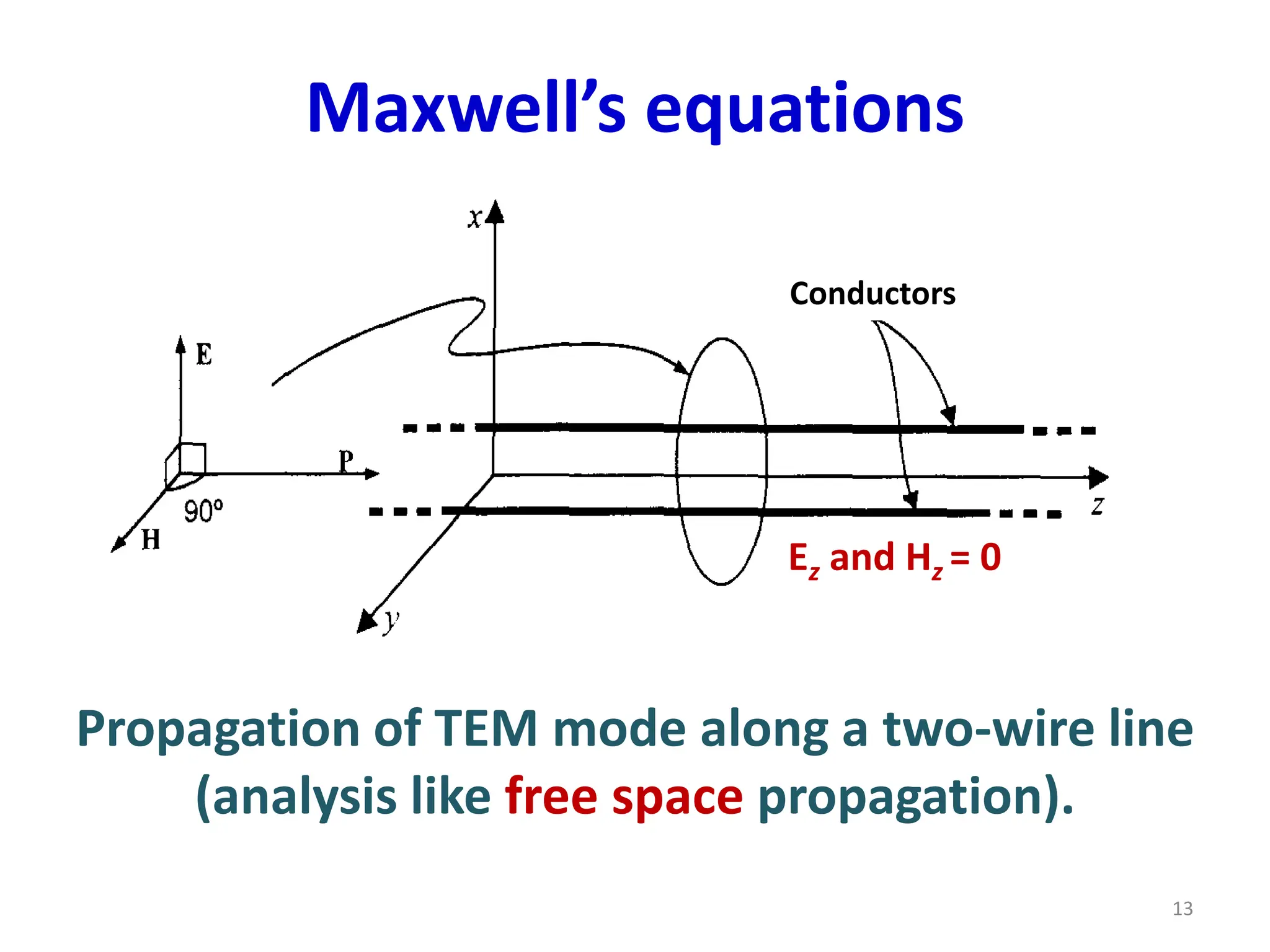
Maxwell’s equations
• Dependingon the region considered
between or around the conductors,
the E field can have the components
Ex and Ey, but always Ez = 0 (equal for
H), so that E and H fields can rotate,
maintaining the perpendicularity
between the two and with the
power flow P always in z direction.
14
15.
Maxwell’s equations
• Thisanalysis is approximate but
valid enough in practice.
• It considers conductors as perfect
and the fields as traveling only
between and around the
conductors.
15
16.
Maxwell’s equations
• Beingrigorous, it would be
necessary to calculate, according to
the f of operation, the depth of
penetration of the fields within the
conductors.
• The resulting distribution of the
waves would no longer be strictly
TEM but quasi or essentially TEM.
16
17.
Maxwell’s equations
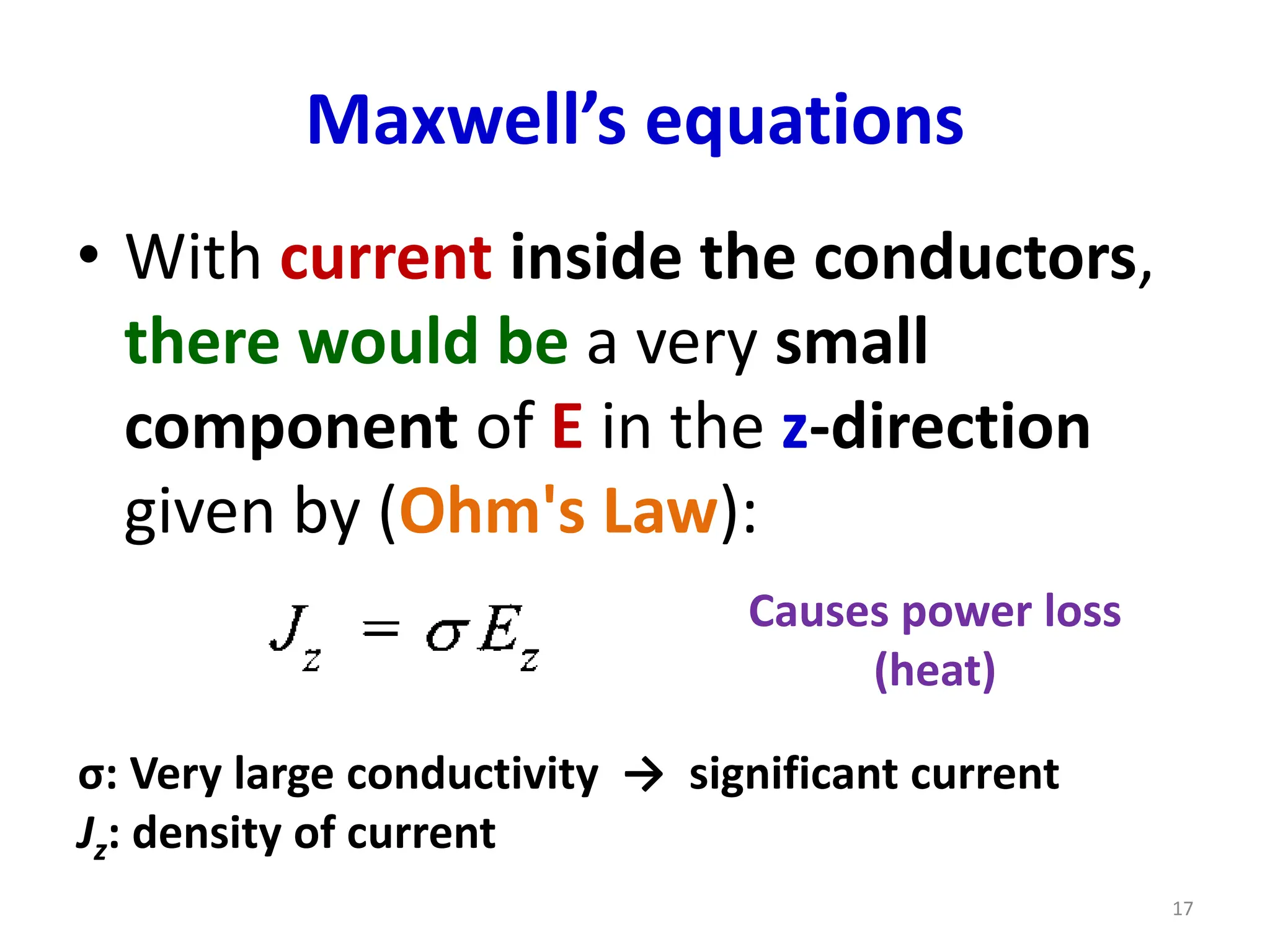
• Withcurrent inside the conductors,
there would be a very small
component of E in the z-direction
given by (Ohm's Law):
Causes power loss
(heat)
σ: Very large conductivity → significant current
Jz: density of current
17
18.
General circuit theory
•Is a simpler method and leads to the
same results.
• This method is preferred in
communications engineering
because it is possible to define and
use the more familiar: voltage V,
current I, and power P variables.
18
19.
General circuit theory
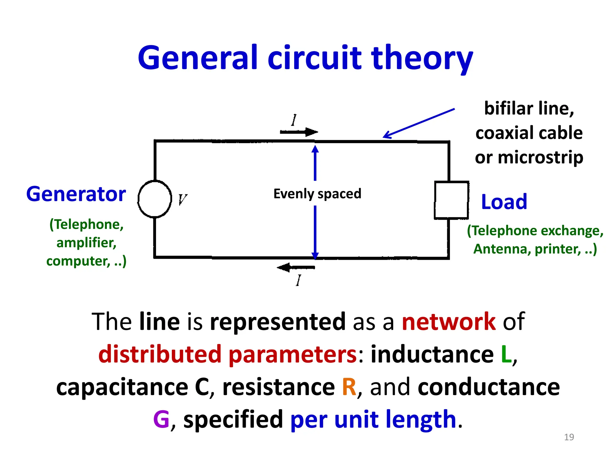
Theline is represented as a network of
distributed parameters: inductance L,
capacitance C, resistance R, and conductance
G, specified per unit length.
bifilar line,
coaxial cable
or microstrip
(Telephone,
amplifier,
computer, ..)
(Telephone exchange,
Antenna, printer, ..)
19
Load
Generator Evenly spaced
20.
Calculation of parameters
•The primary parameters of the line
(L, C, R, and G) can be calculated for
every case provided that
dimensions and operation
frequency are known.
• As neither the conductors nor the
dielectric are perfect (R is added in
series and G in parallel).
20
21.
Calculation of parameters
•Inductance (L), is a measure of the
opposition to the changes in the
amount of current in an inductor or
coil that stores energy in the
presence of a magnetic field.
21
22.
Calculation of parameters
•Inductance is defined as the
relationship between the magnetic
flow (Φ) and the electric current
intensity (I) circulating through the
coil for several turns (N) of the
winding:
L = NΦ/I
22
23.
Calculation of parameters
•The inductance depends on the
physical characteristics of the electric
conductor and of its length. It appears
when an electric conductor is rolled
up.
• The more turns, the more inductance.
• It increases by adding a ferrite core.
23
24.
Calculation of parameters
•Capacitance (C) is the property of a
capacitor to oppose to any variation of
the voltage in the electrical circuit.
• Is the ability of a system to store an
electric charge. It appears between
two isolated conductors when there is
an electric potential difference
between them.
24
25.
Calculation of parameters
•Capacitance is calculated as the ratio
between the electric charge Q on
each conductor and the electrical
potential difference V.
C = Q/V
25
26.
Calculation of parameters
•C only depends on the physical
dimensions and geometry of the
line, while L is a function of current
distribution.
• At low frequencies, the current
flows on the surface and inside the
conductor, at very high frequencies
it goes only on the surface.
26
27.
Calculation of parameters
•As the conductors are not perfect, it
should be considered a resistance R
in series.
• The dielectric between the
conductors is also not perfect and
should be considered a conductance
G in parallel (allows leaks or electric
arcs).
27
28.
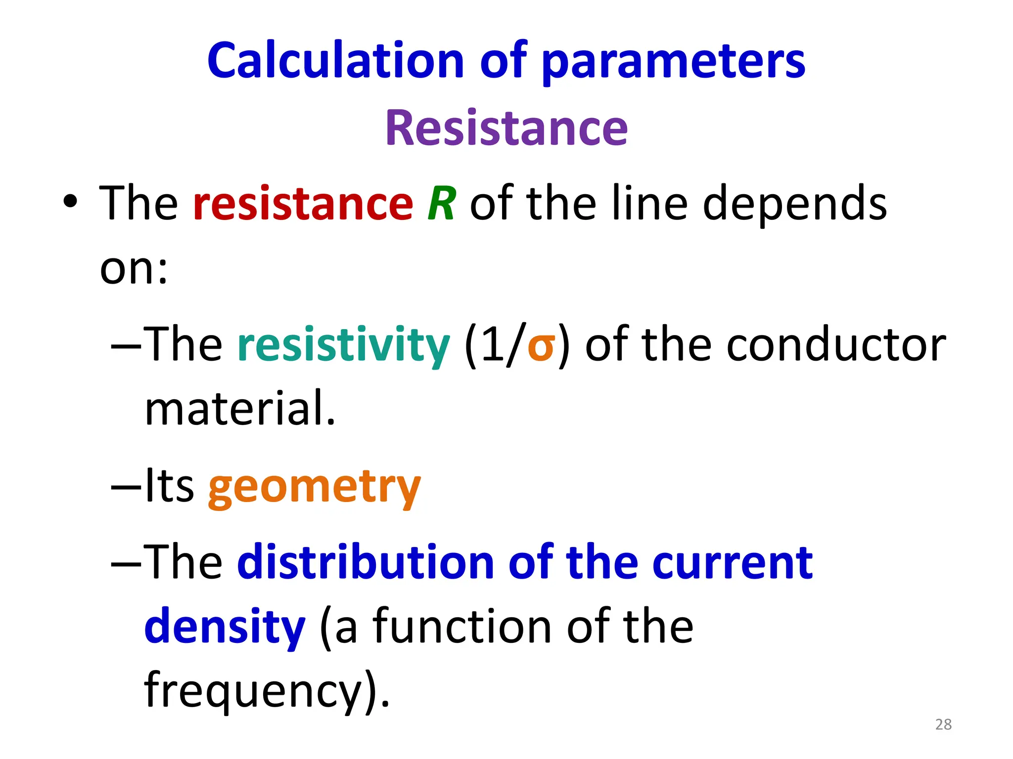
Calculation of parameters
Resistance
•The resistance R of the line depends
on:
–The resistivity (1/σ) of the conductor
material.
–Its geometry
–The distribution of the current
density (a function of the
frequency). 28
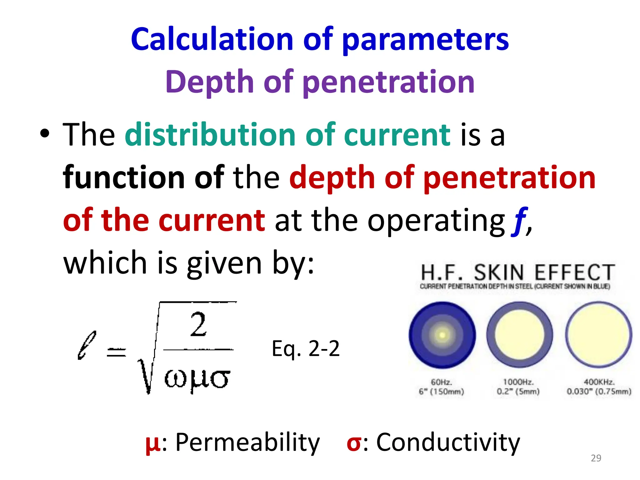
29.
Calculation of parameters
Depthof penetration
• The distribution of current is a
function of the depth of penetration
of the current at the operating f,
which is given by:
μ: Permeability σ: Conductivity
Eq. 2-2
29
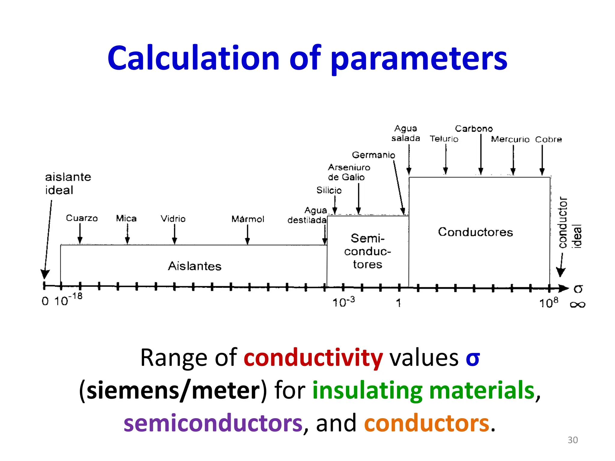
30.
Calculation of parameters
Rangeof conductivity values σ
(siemens/meter) for insulating materials,
semiconductors, and conductors. 30
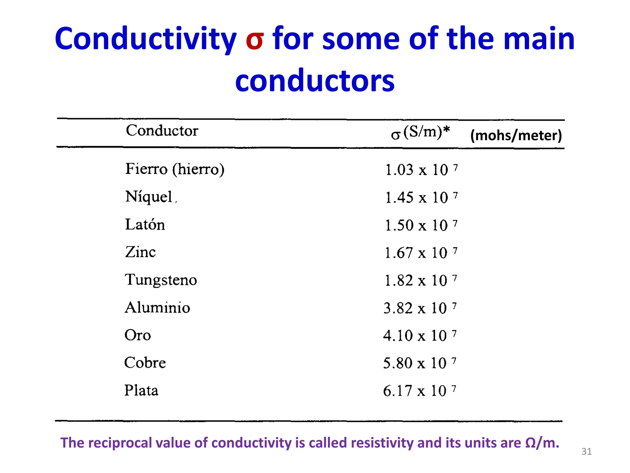
31.
Conductivity σ forsome of the main
conductors
(mohs/meter)
The reciprocal value of conductivity is called resistivity and its units are Ω/m. 31
32.
Calculation of parameters
Conductance
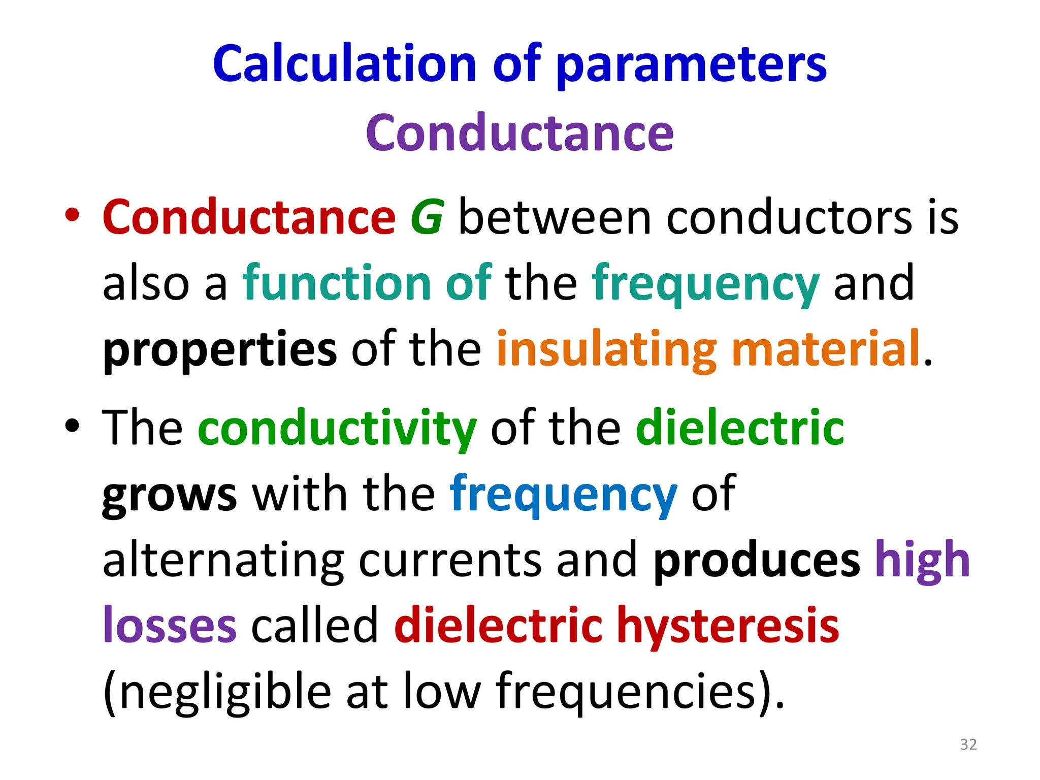
•Conductance G between conductors is
also a function of the frequency and
properties of the insulating material.
• The conductivity of the dielectric
grows with the frequency of
alternating currents and produces high
losses called dielectric hysteresis
(negligible at low frequencies).
32
33.
Dielectric hysteresis
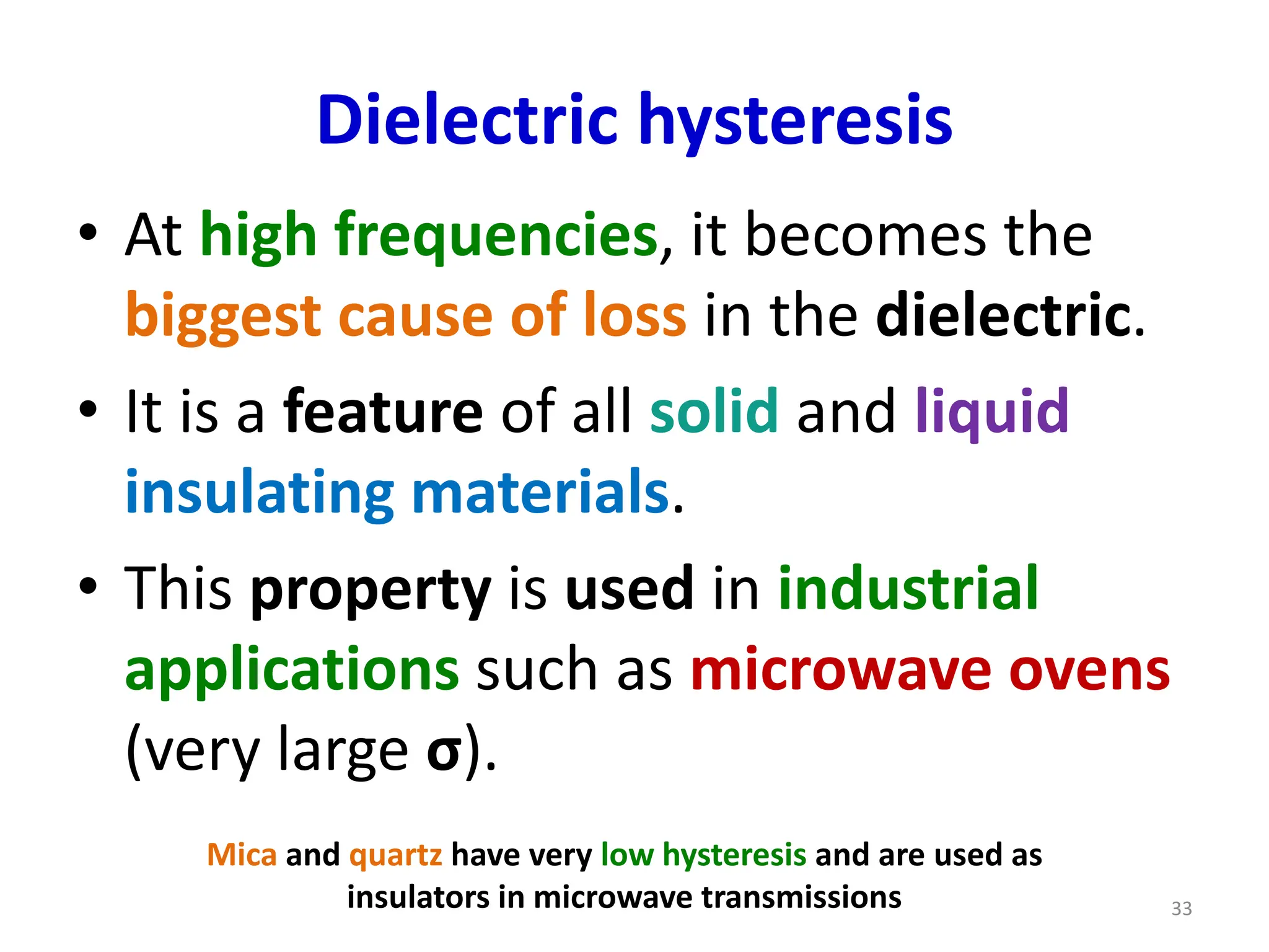
• Athigh frequencies, it becomes the
biggest cause of loss in the dielectric.
• It is a feature of all solid and liquid
insulating materials.
• This property is used in industrial
applications such as microwave ovens
(very large σ).
Mica and quartz have very low hysteresis and are used as
insulators in microwave transmissions 33
34.
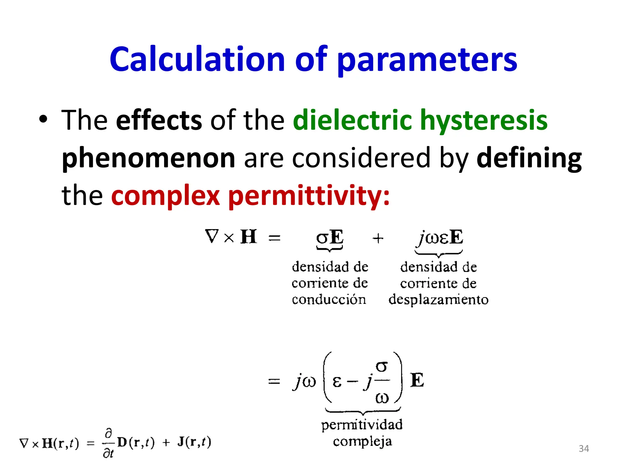
Calculation of parameters
•The effects of the dielectric hysteresis
phenomenon are considered by defining
the complex permittivity:
34
35.
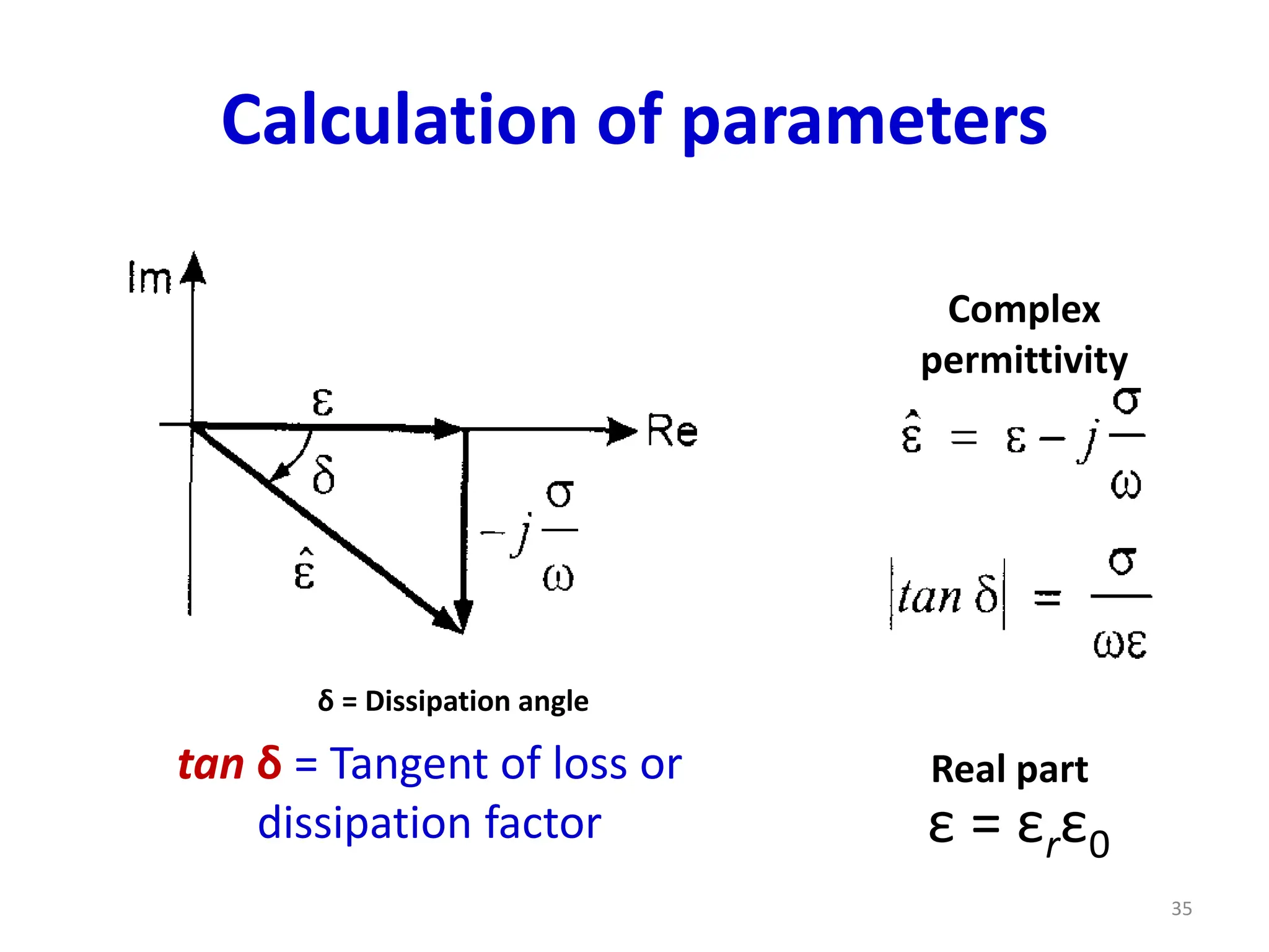
Calculation of parameters
ε= εrε0
tan δ = Tangent of loss or
dissipation factor
Complex
permittivity
Real part
35
δ = Dissipation angle
36.
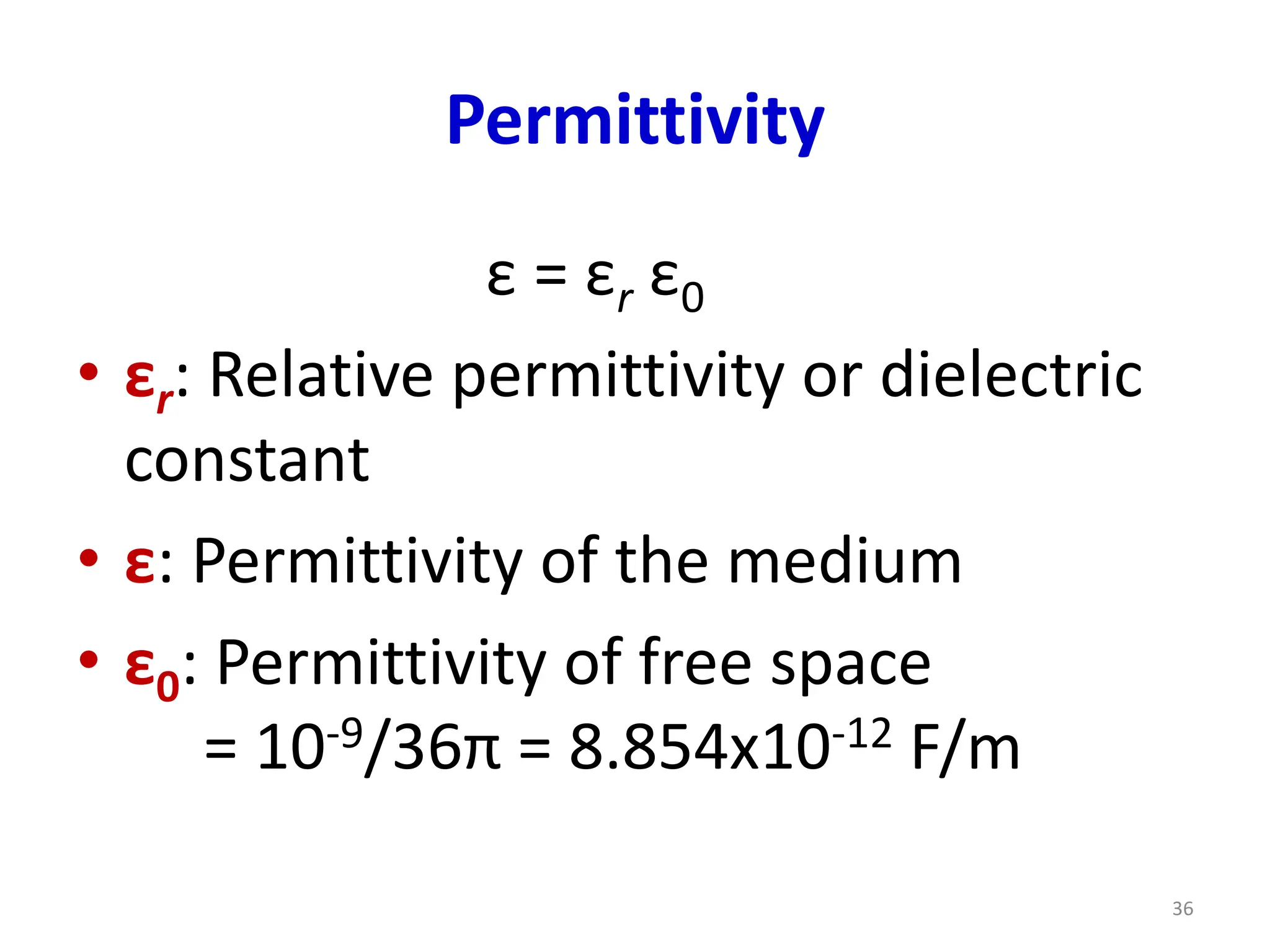
Permittivity
ε = εrε0
• εr: Relative permittivity or dielectric
constant
• ε: Permittivity of the medium
• ε0: Permittivity of free space
= 10-9/36π = 8.854x10⁻¹² F/m
36
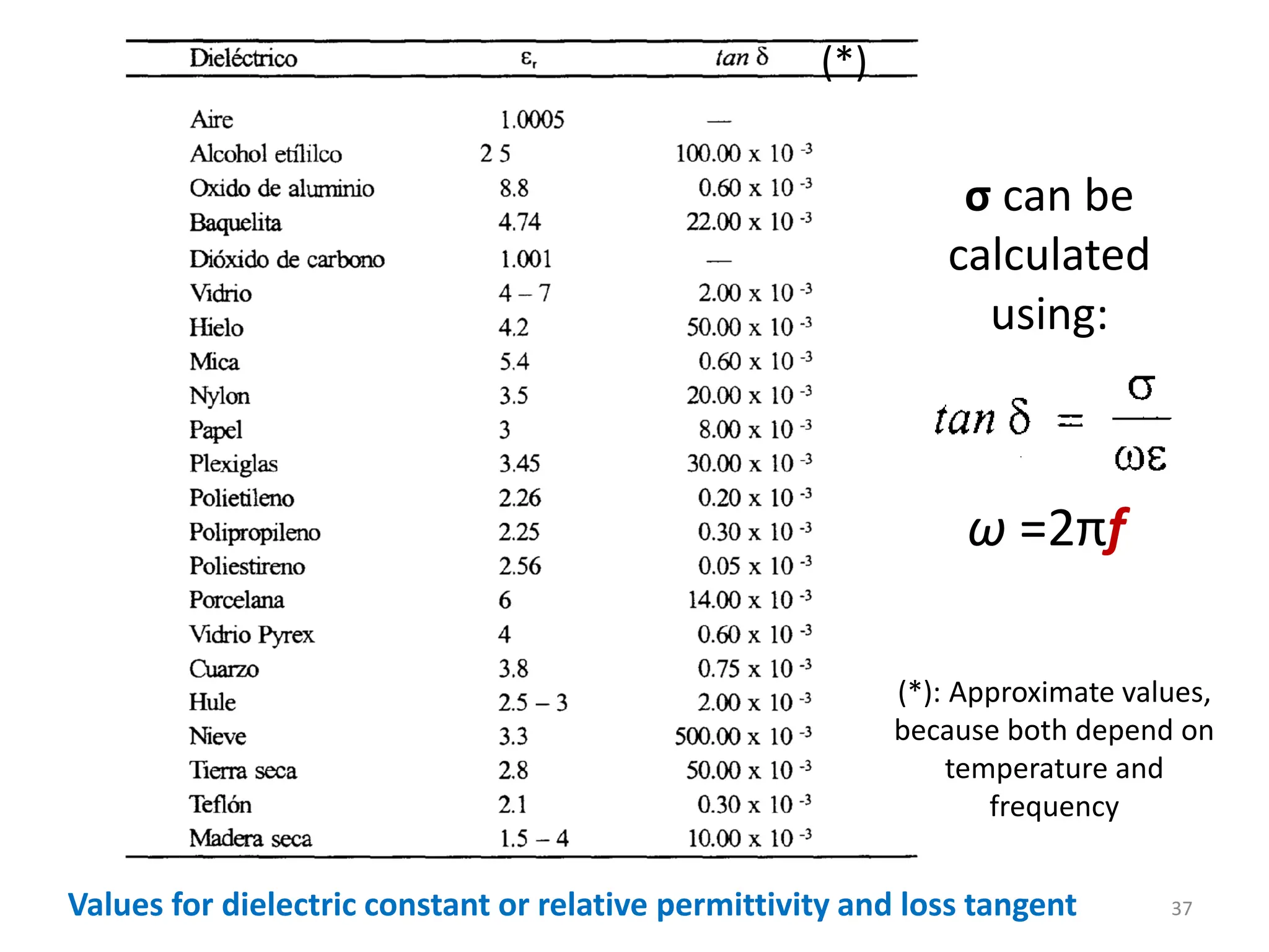
37.
Values for dielectricconstant or relative permittivity and loss tangent
ω =2πf
σ can be
calculated
using:
(*)
(*): Approximate values,
because both depend on
temperature and
frequency
37
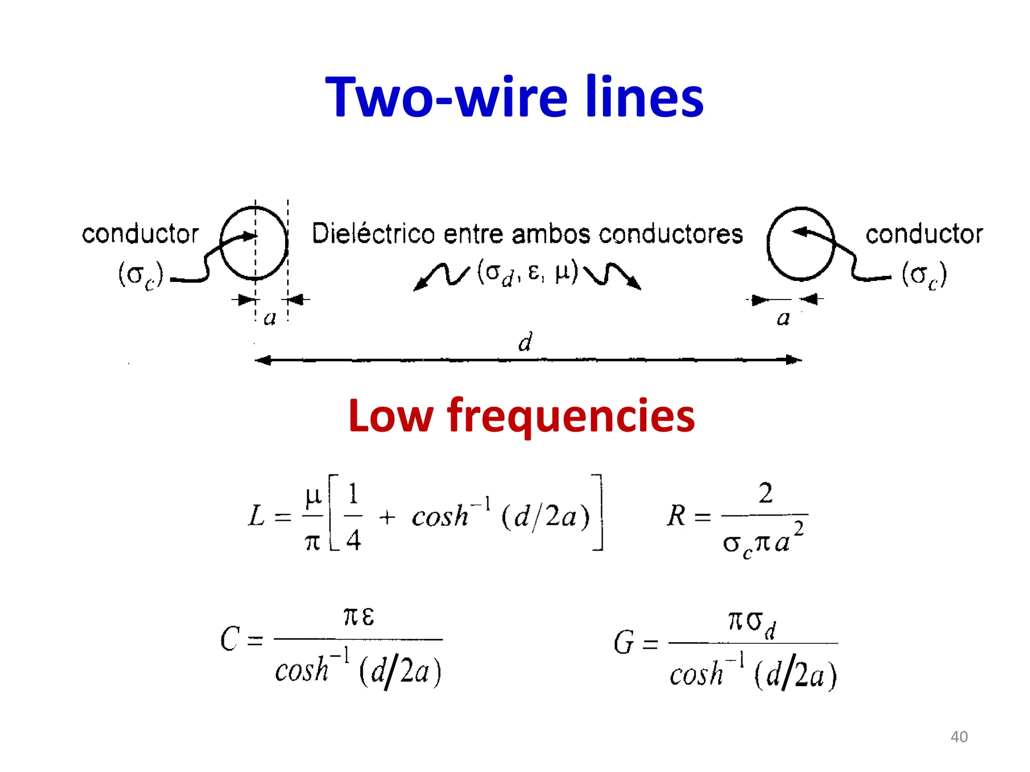
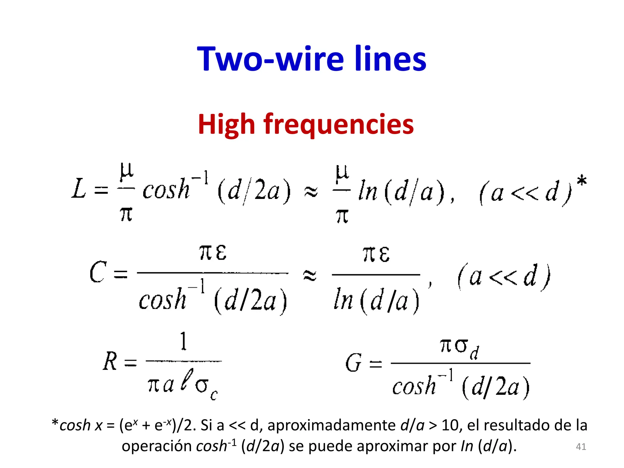
Two-wire lines
High frequencies
*coshx = (ex + e-x)/2. Si a << d, aproximadamente d/a > 10, el resultado de la
operación cosh-1 (d/2a) se puede aproximar por In (d/a). 41
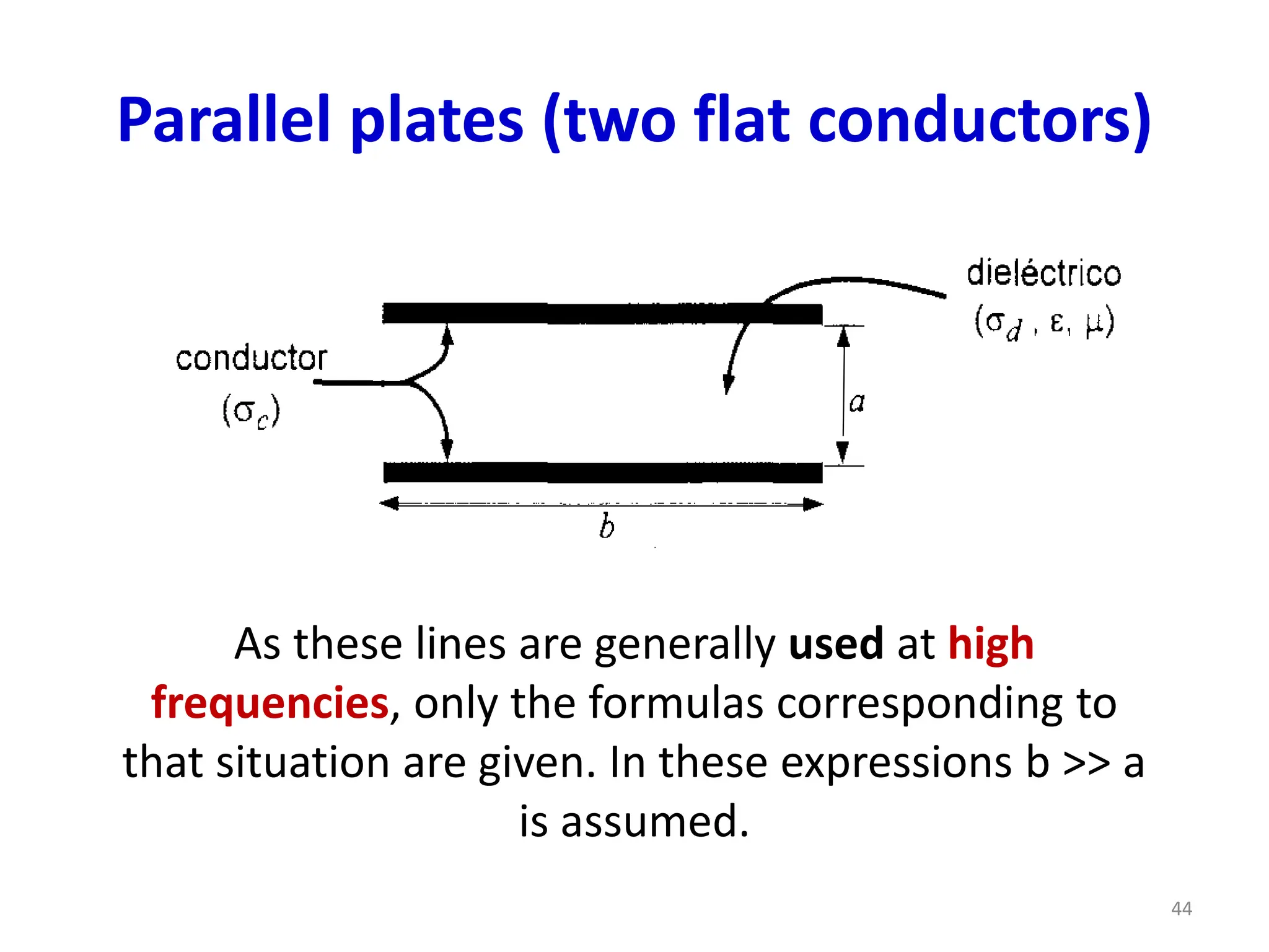
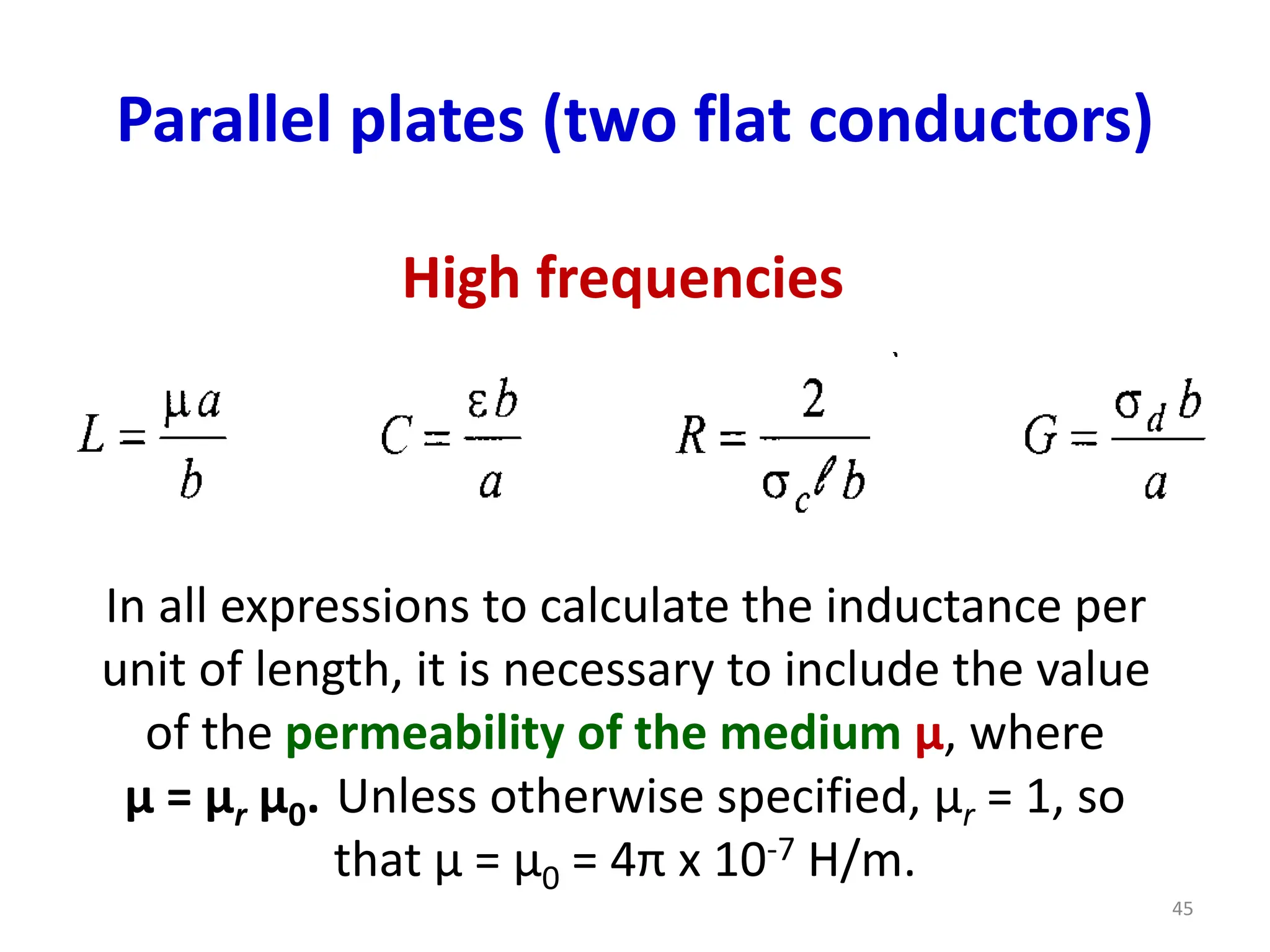
Parallel plates (twoflat conductors)
As these lines are generally used at high
frequencies, only the formulas corresponding to
that situation are given. In these expressions b >> a
is assumed.
44
45.
Parallel plates (twoflat conductors)
High frequencies
In all expressions to calculate the inductance per
unit of length, it is necessary to include the value
of the permeability of the medium μ, where
μ = μr μ0. Unless otherwise specified, μr = 1, so
that μ = μ0 = 4π x 10-7 H/m.
45
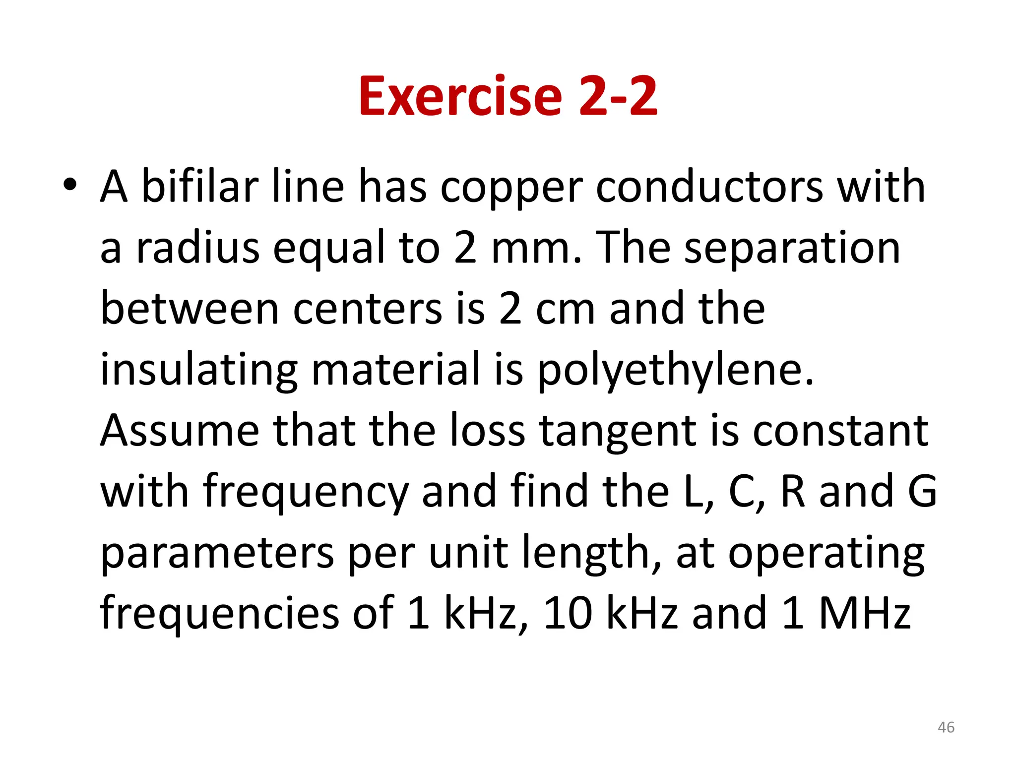
46.
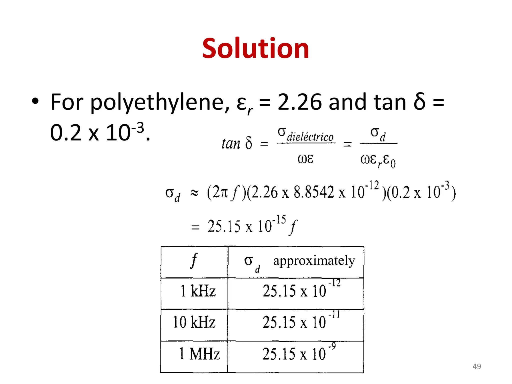
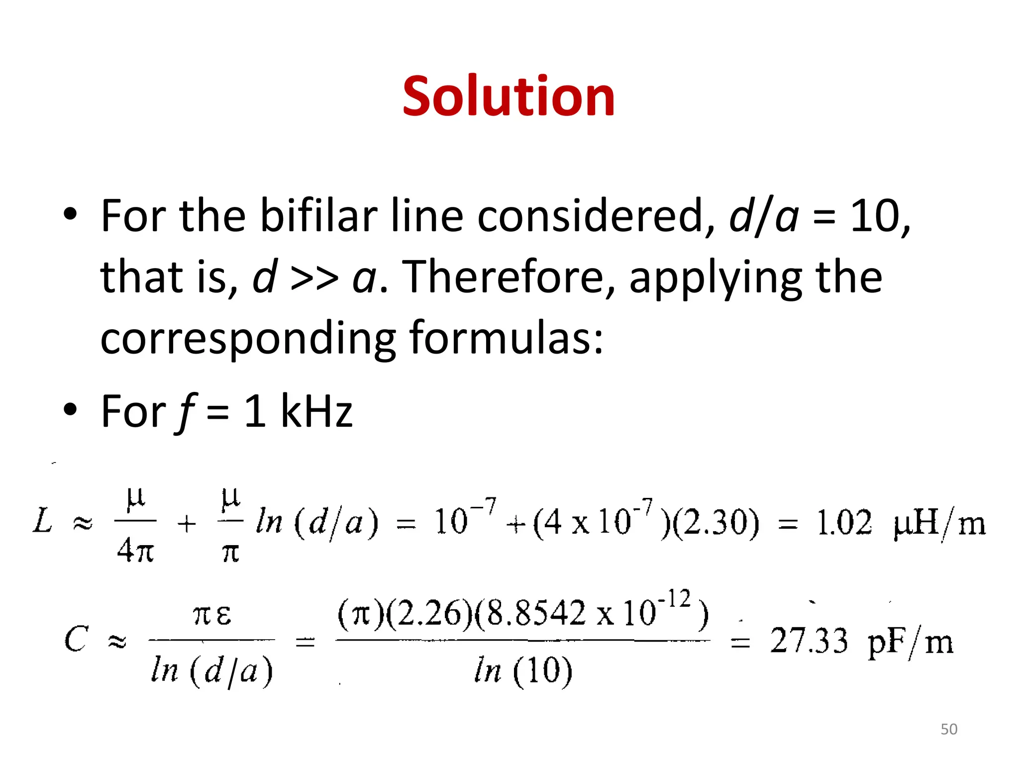
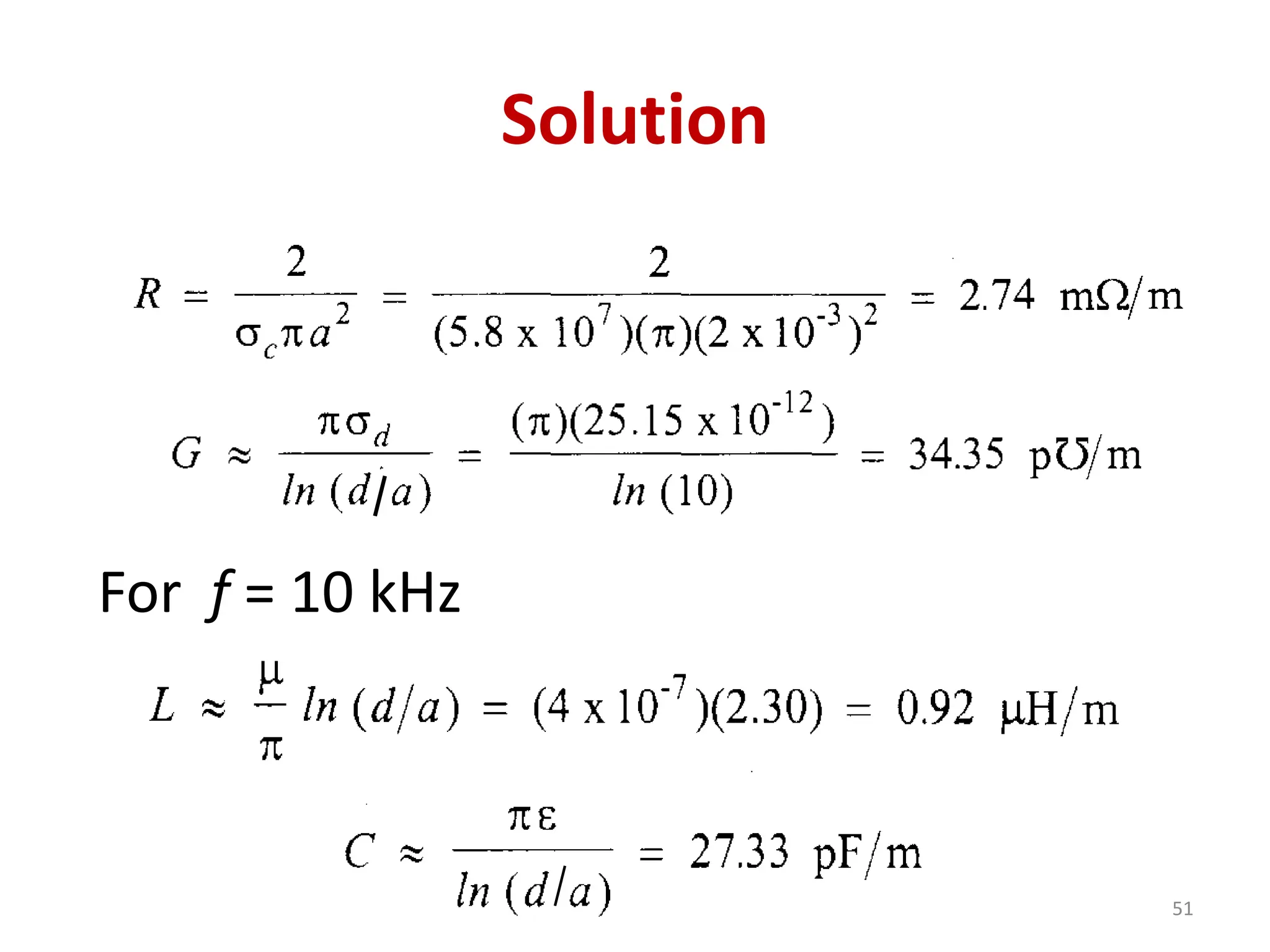
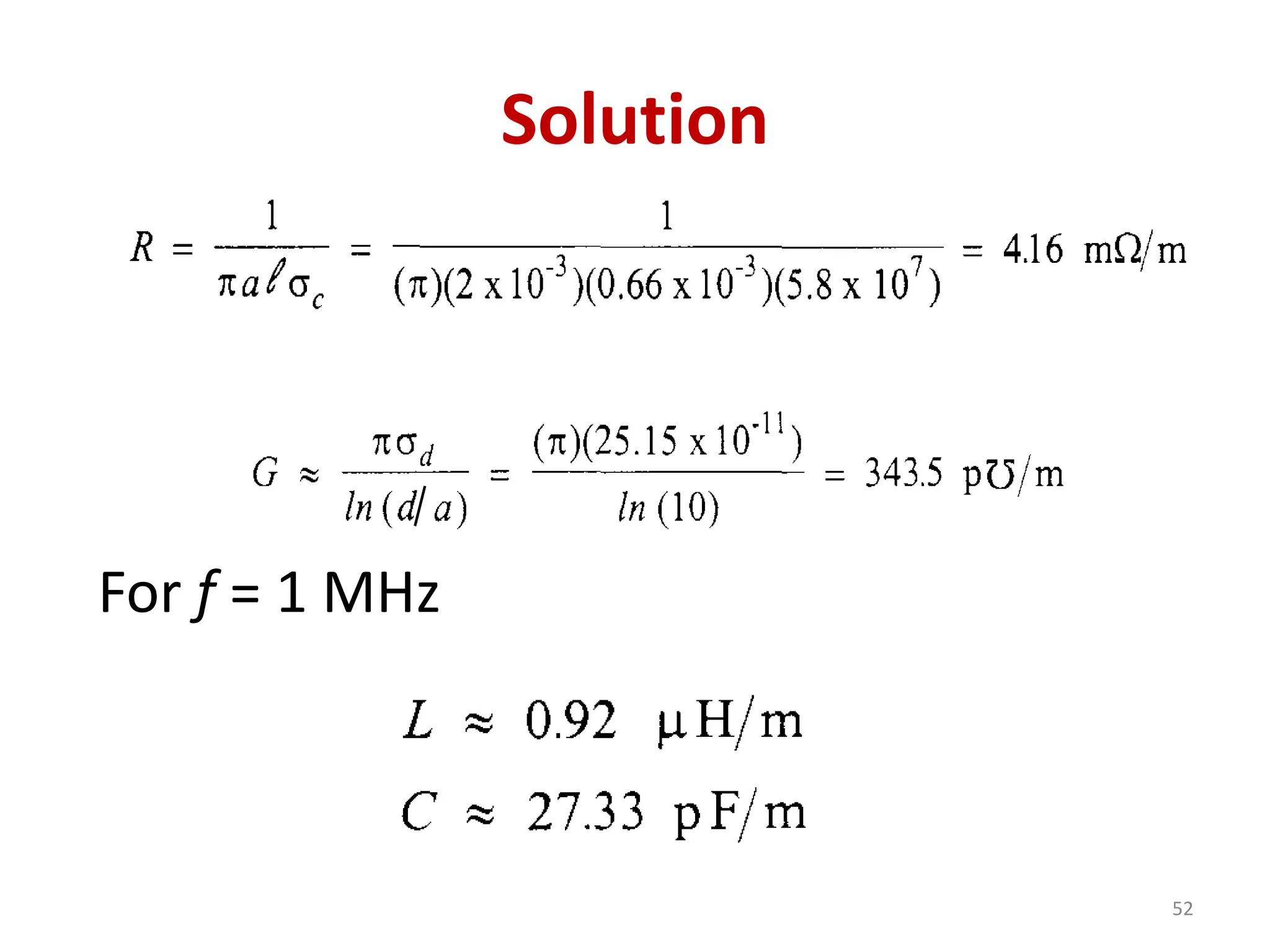
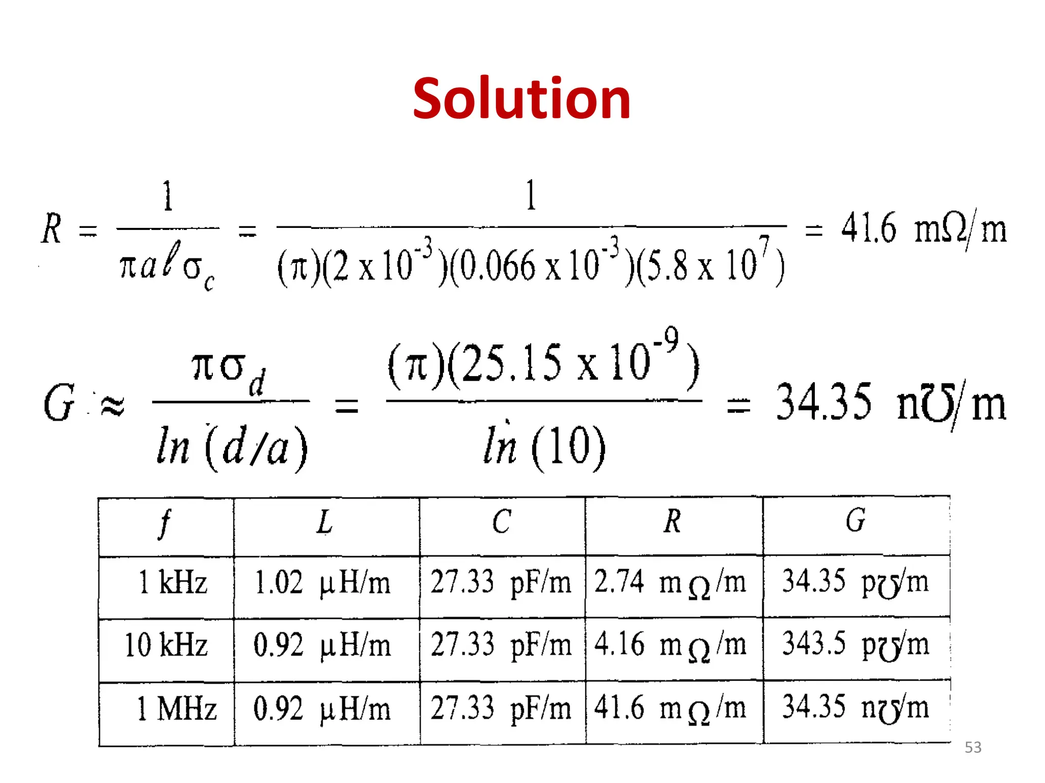
Exercise 2-2
• Abifilar line has copper conductors with
a radius equal to 2 mm. The separation
between centers is 2 cm and the
insulating material is polyethylene.
Assume that the loss tangent is constant
with frequency and find the L, C, R and G
parameters per unit length, at operating
frequencies of 1 kHz, 10 kHz and 1 MHz
46
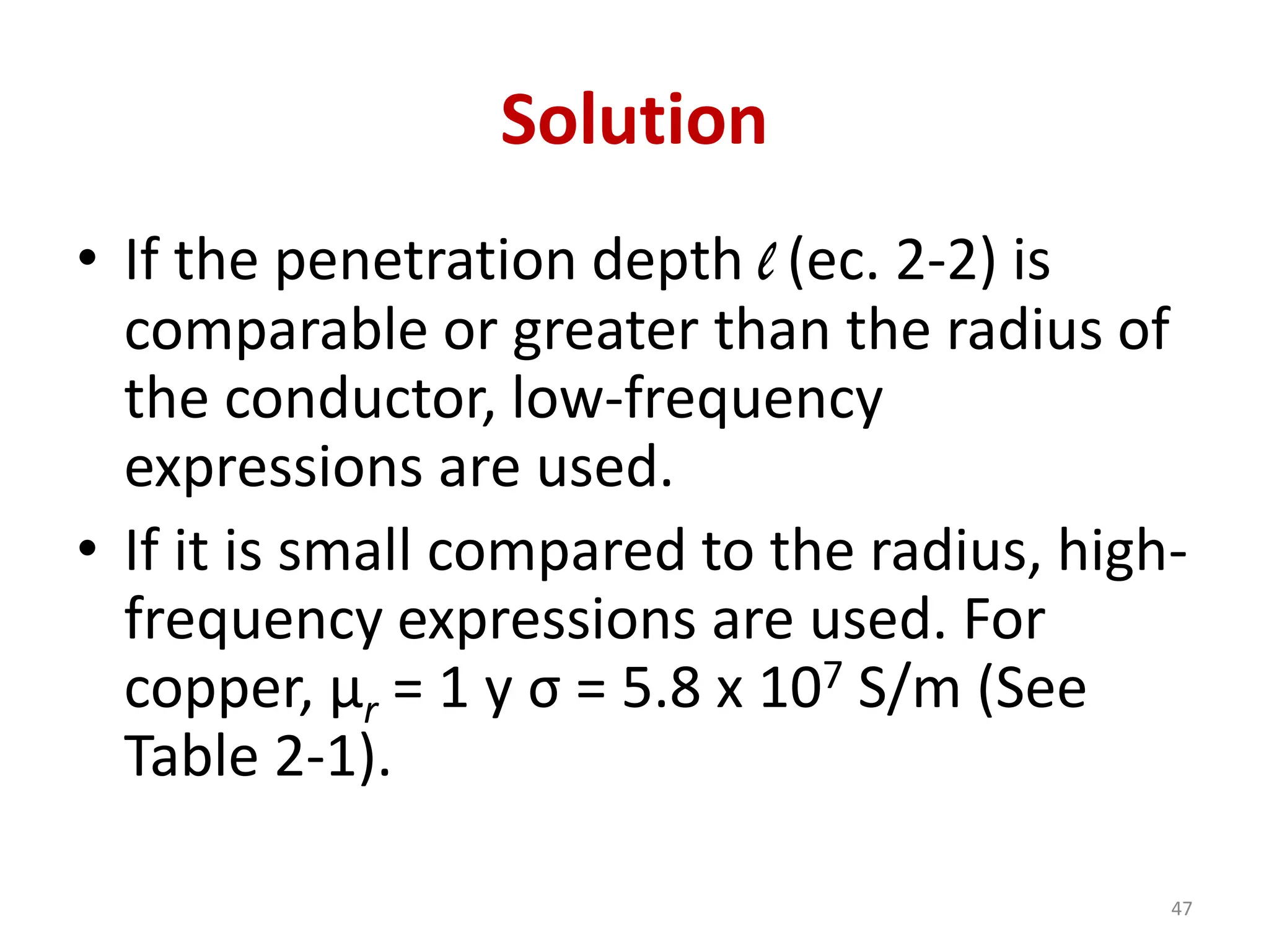
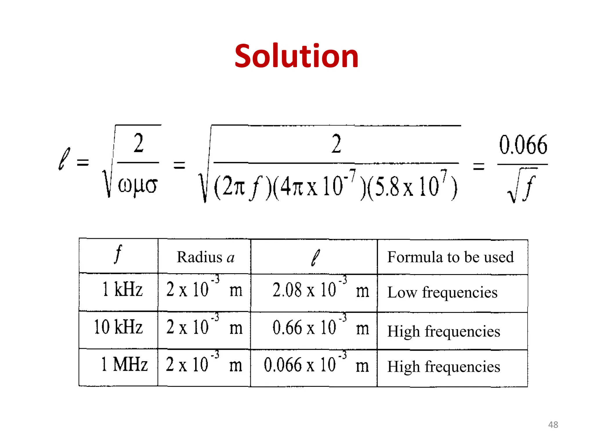
47.
Solution
• If thepenetration depth l (ec. 2-2) is
comparable or greater than the radius of
the conductor, low-frequency
expressions are used.
• If it is small compared to the radius, high-
frequency expressions are used. For
copper, μr = 1 y σ = 5.8 x 10⁷ S/m (See
Table 2-1).
47
Conclusions
• C isindependent of f, as is L (from a
certain intermediate f).
• This is inferred by observation and
comparison of the corresponding
equations for low and high
frequencies.
54
55.
Conclusions
• R andG increase with f.
• This is because as f is higher, the film
effect of the current on the conductors is
more marked.
• The effective area through which the
current is distributed is smaller and
therefore the resistance increases in
proportion to the square root of the
working frequency.
55
56.
Conclusions
• The increaseof G with f is directly
proportional to the increase of the σ
of the dielectric due to the
phenomenon of hysteresis (it can
also be inferred by observation of
the corresponding equations).
56
57.
Exercise 2-3
• Considera coaxial cable designed to
operate at very high temperatures, for
example on rockets, missiles and
satellites.
• The dielectric between both copper
conductors is Teflon and the walls that
contact such dielectric are coated in
silver.
57
58.
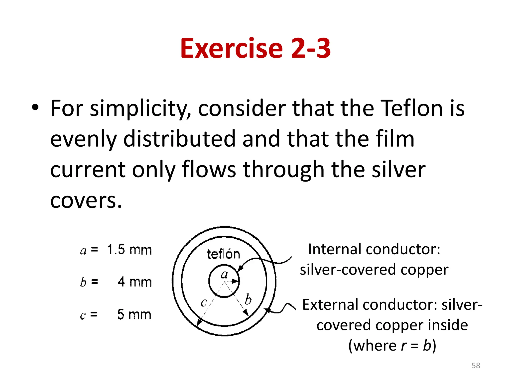
Exercise 2-3
• Forsimplicity, consider that the Teflon is
evenly distributed and that the film
current only flows through the silver
covers.
58
Internal conductor:
silver-covered copper
External conductor: silver-
covered copper inside
(where r = b)
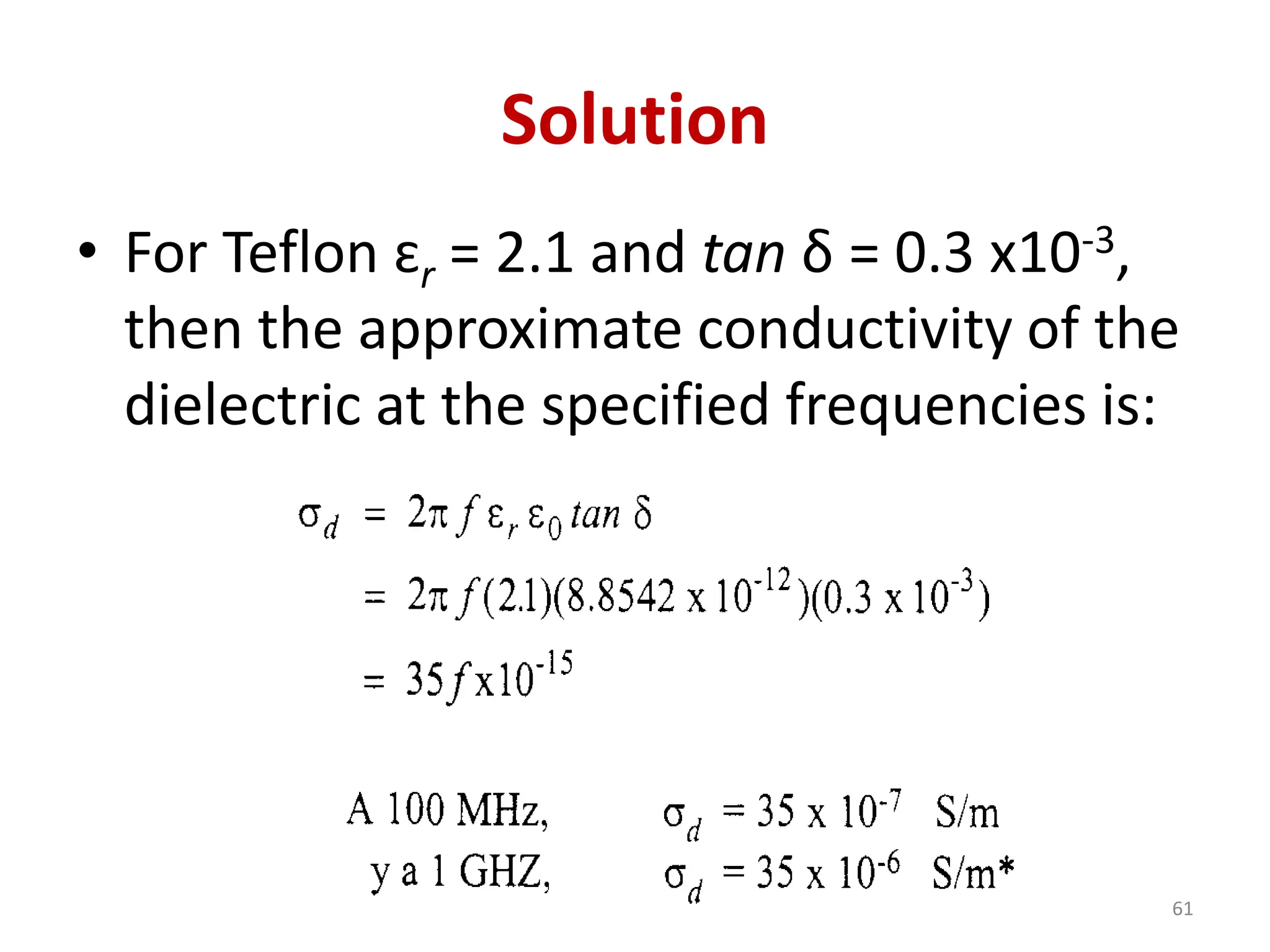
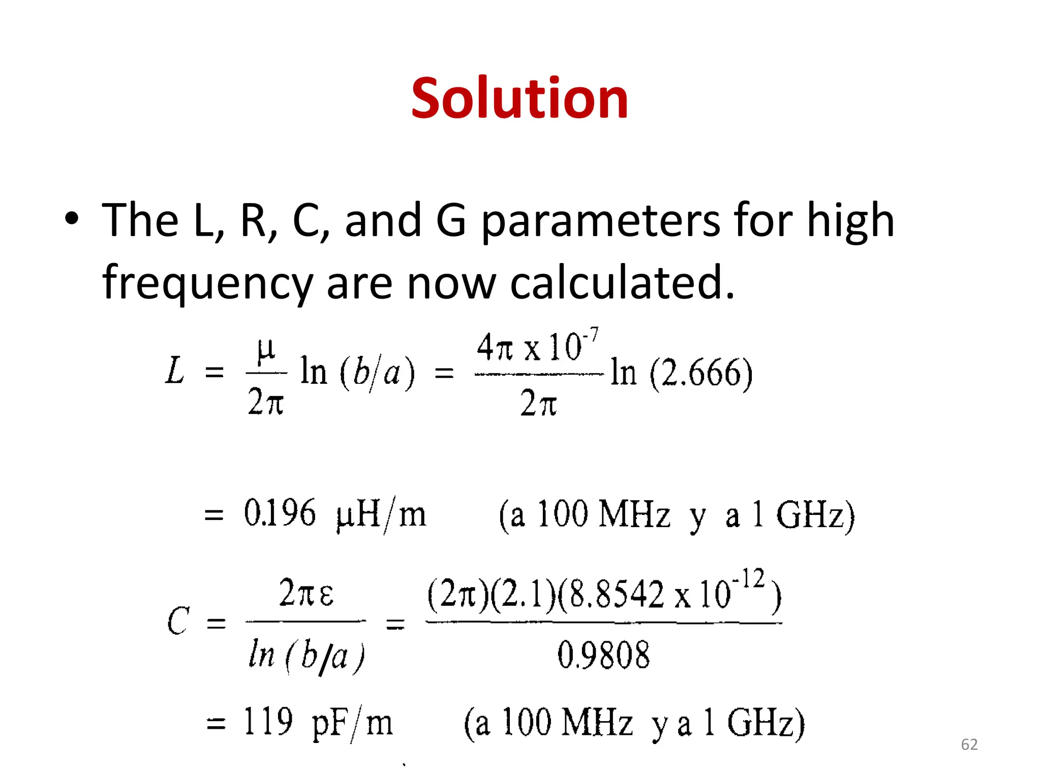
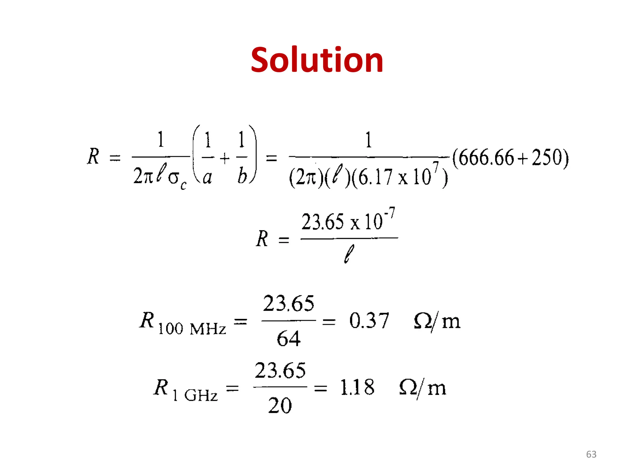
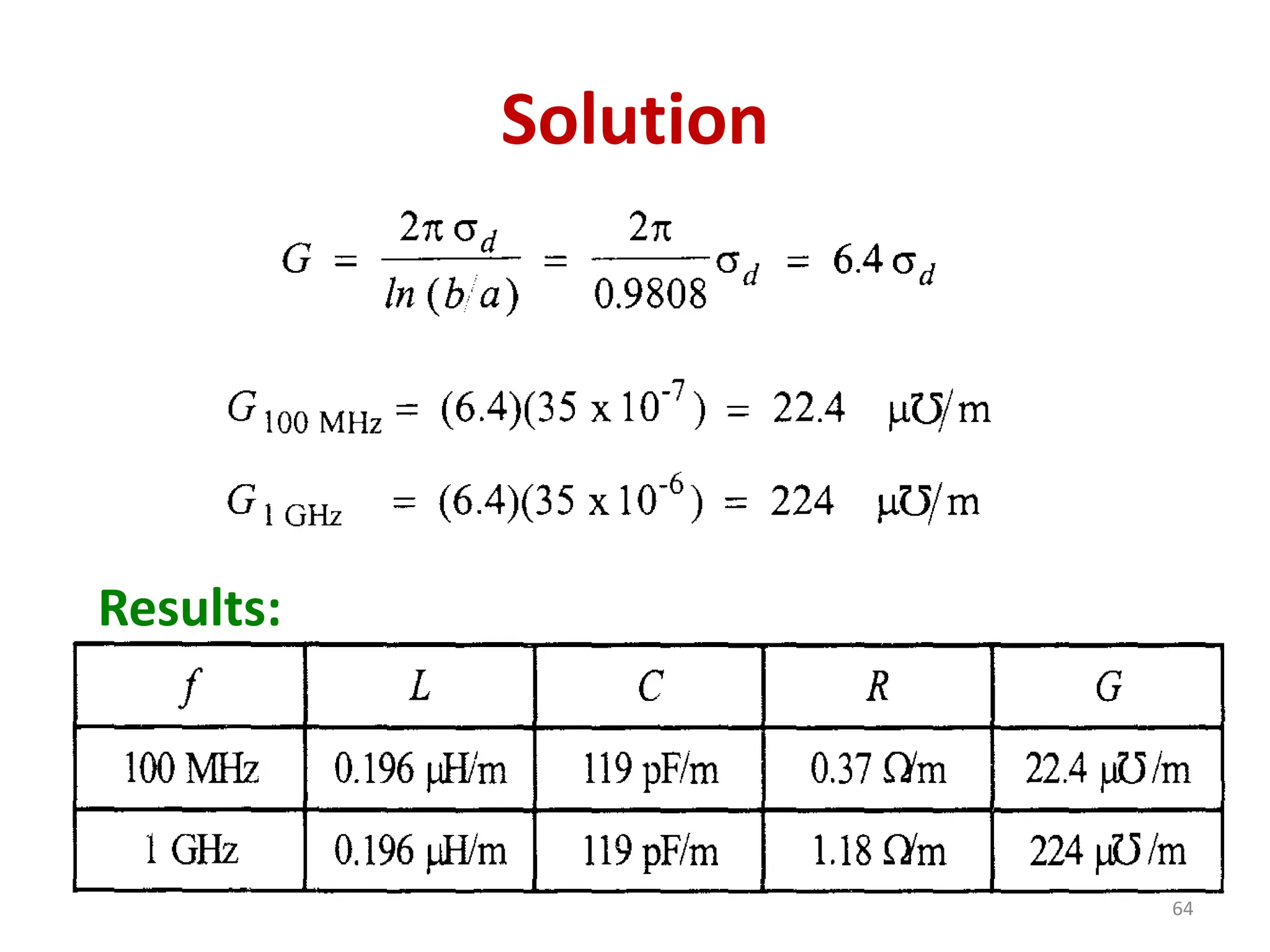
59.
Exercise 2-3
• CalculateL, C, R, and G parameters for
this line at 100 MHz and 1 GHz.
Solution
• First, the depth of penetration l is
estimated to confirm the validity of the
assumption that current flows on the
silver layer only.
59
Suggested exercise
• Aninternal telephone line used to connect the
phone box to the outside network, consists of
two parallel copper conductors with a
diameter of 0.60 mm. The separation between
the conductor centers is 2.5 mm and the
insulating material between the two is
polyethylene. Calculate the L, C, R, and G
parameters per unit length at a frequency of 3
kHz.
[L = 942nH/m, C = 30 pF/m, R = 122 mΩ/m, G = 112 pƱ/m].
65
Introduction
• Knowing thebasic parameters of a
line it is possible to determine the
relationship between the voltage
and current waves that travel along
it, from the generator to the load, as
well as the speed with which they do
so.
67
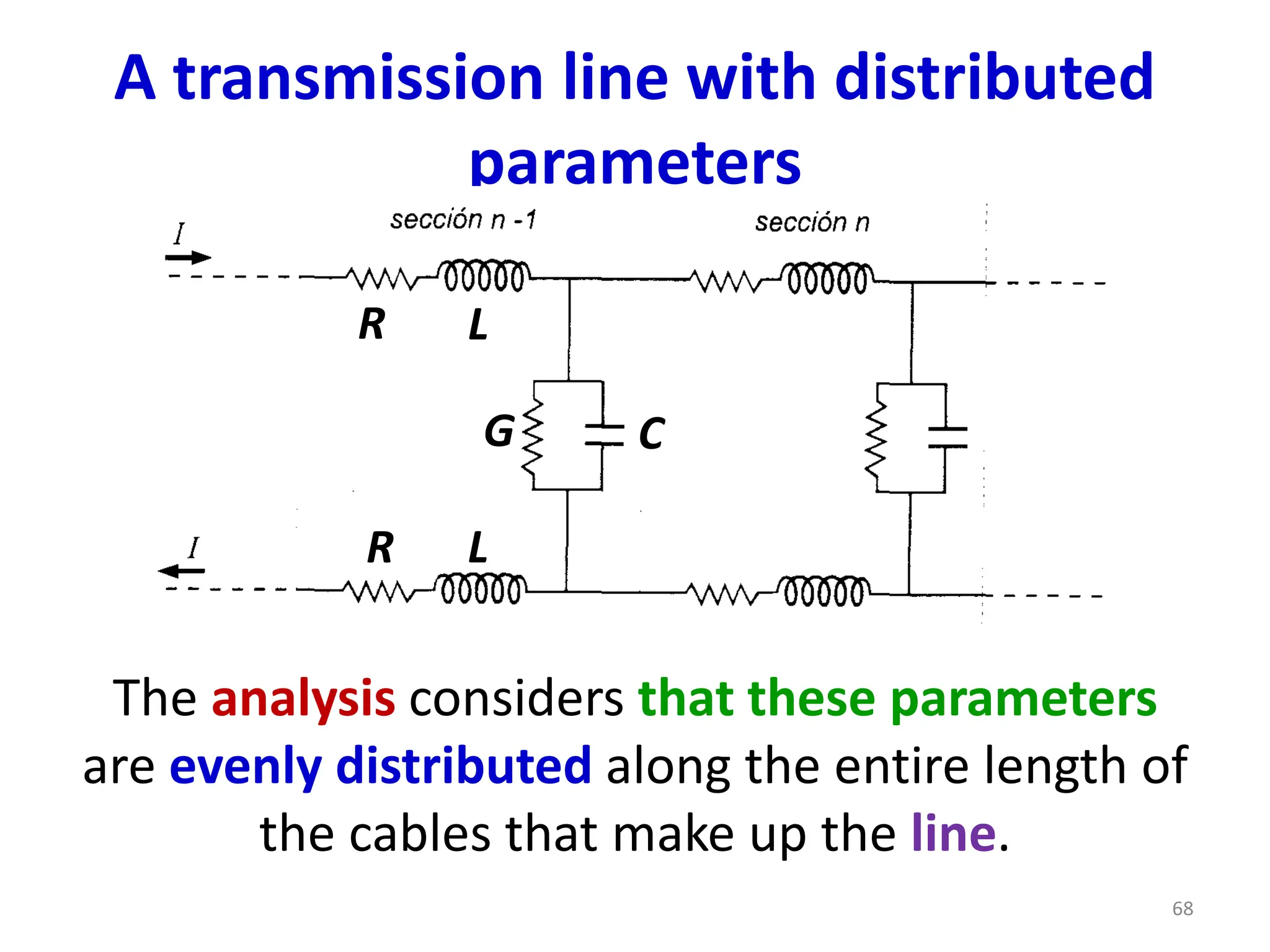
68.
A transmission linewith distributed
parameters
The analysis considers that these parameters
are evenly distributed along the entire length of
the cables that make up the line.
R L
G C
R L
68
69.
Distributed parameters
• Thetransmission line with
distributed parameters can be
represented by an equivalent circuit
composed of many resistors and
inductances in series and many
conductances and capacitances in
parallel.
69
70.
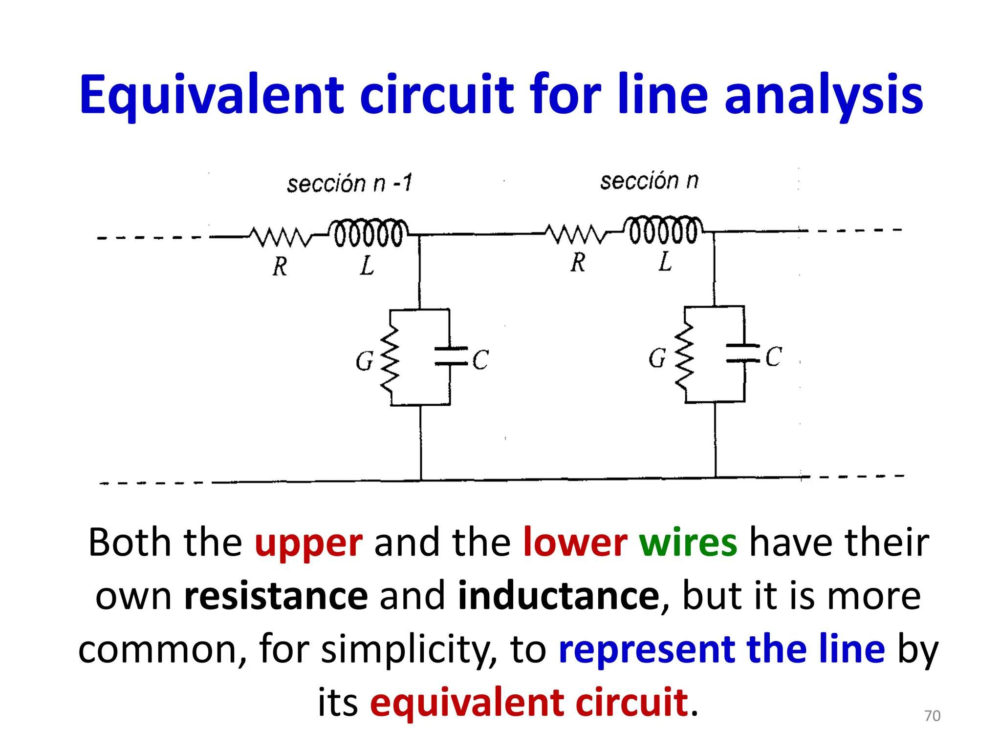
Equivalent circuit forline analysis
Both the upper and the lower wires have their
own resistance and inductance, but it is more
common, for simplicity, to represent the line by
its equivalent circuit. 70
71.
Equivalent circuit
• Thereare other possible
representations, such as the
equivalent T circuit or the π circuit,
depending on how C and G are
considered located in each section.
• Any of these equivalent circuits will
lead to the same mathematical
expressions.
71
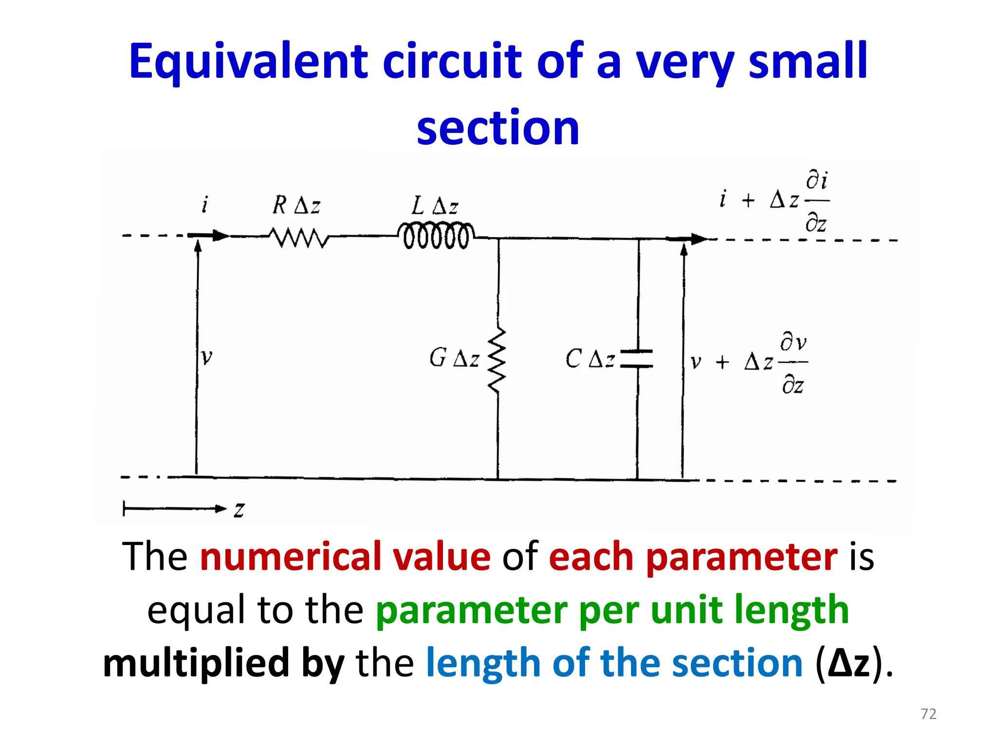
72.
Equivalent circuit ofa very small
section
The numerical value of each parameter is
equal to the parameter per unit length
multiplied by the length of the section (Δz).
72
73.
Equivalent circuit ofa very small
section
• Current i and voltage v are functions of
both distance z and time t, so that at the
end of the section considered there are
increases in current and voltage.
• If Δz is made to tend to zero (Δz → 0),
the same symmetry and results are
obtained as with an equivalent T or π
circuit.
73
74.
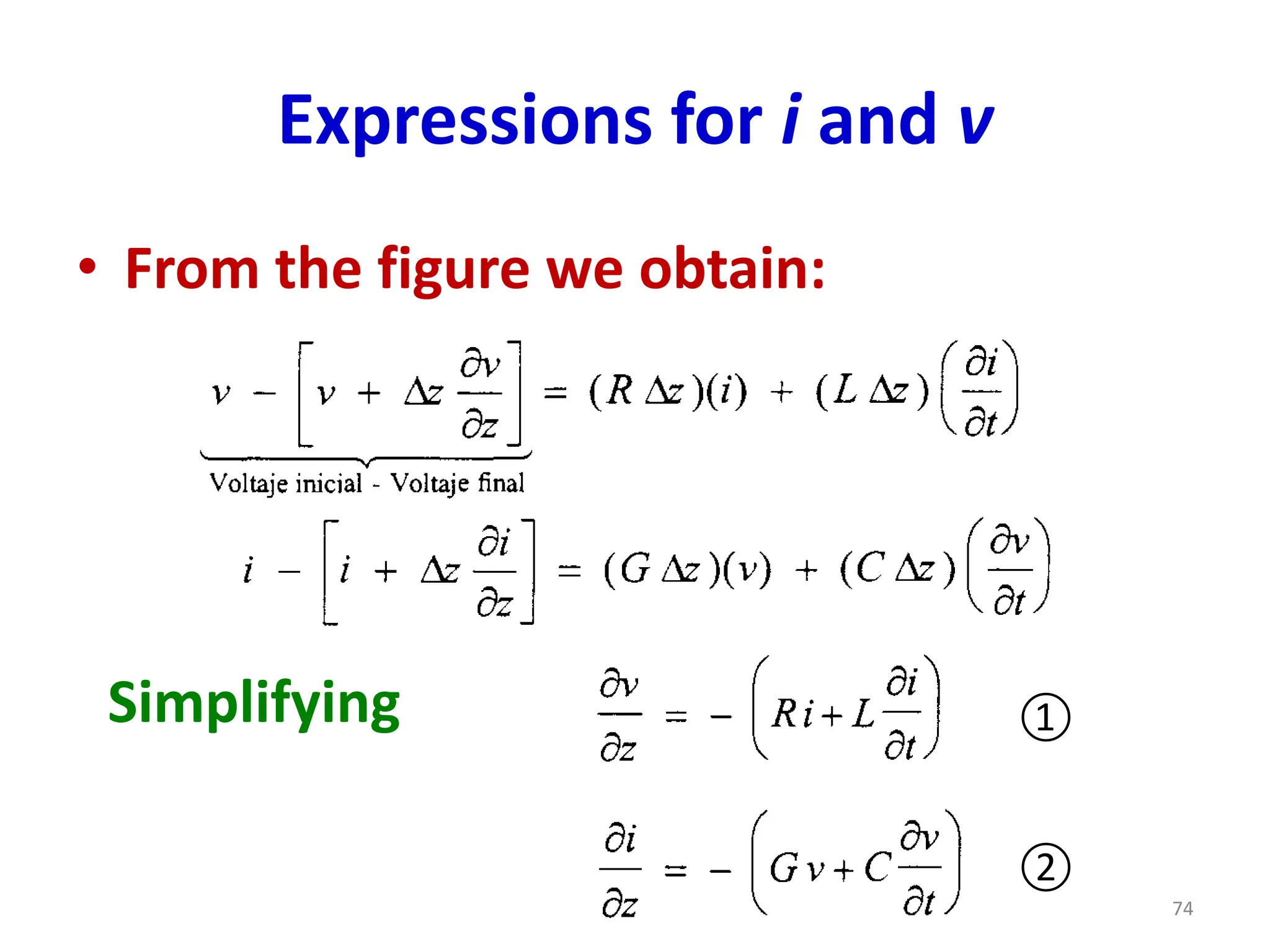
Expressions for iand v
• From the figure we obtain:
Simplifying ①
②
74
75.
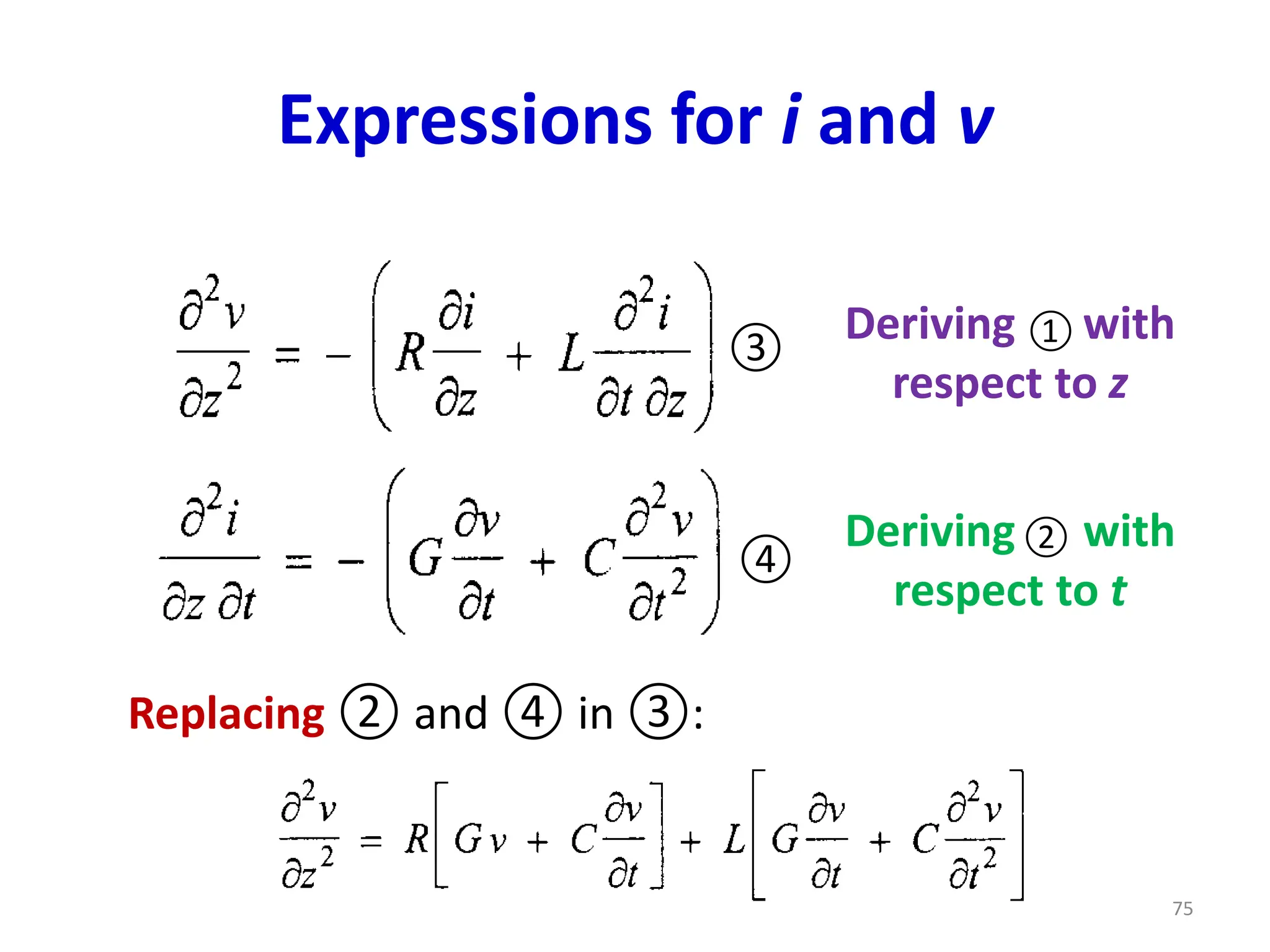
Expressions for iand v
Deriving with
respect to z
Deriving with
respect to t
③
④
Replacing ② and ④ in ③:
75
①
②
76.
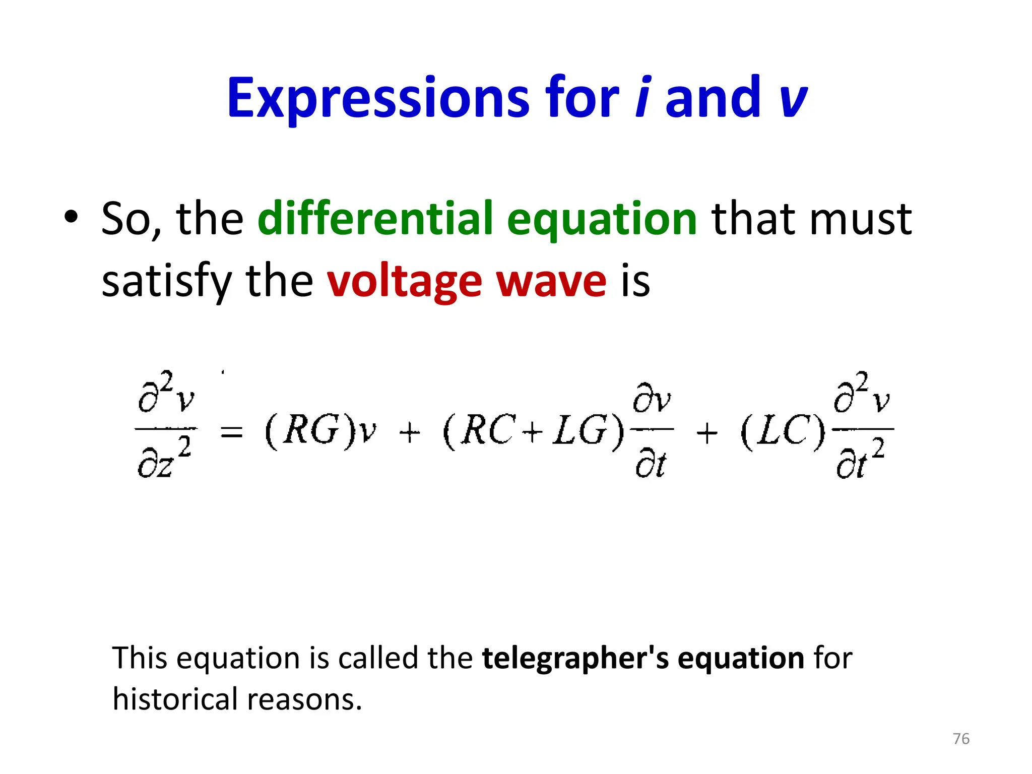
Expressions for iand v
• So, the differential equation that must
satisfy the voltage wave is
This equation is called the telegrapher's equation for
historical reasons.
76
77.
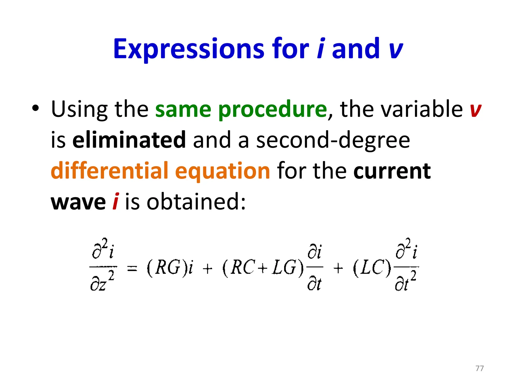
Expressions for iand v
• Using the same procedure, the variable v
is eliminated and a second-degree
differential equation for the current
wave i is obtained:
77
78.
Expressions for iand v
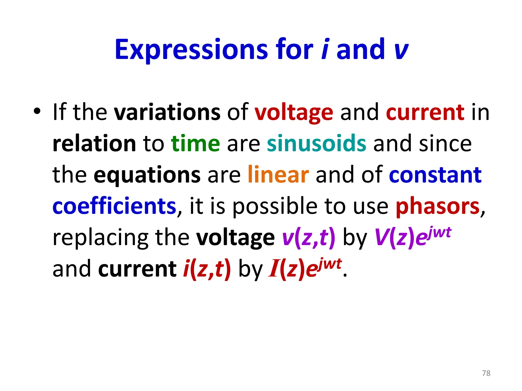
• If the variations of voltage and current in
relation to time are sinusoids and since
the equations are linear and of constant
coefficients, it is possible to use phasors,
replacing the voltage v(z,t) by V(z)ejwt
and current i(z,t) by I(z)ejwt.
78
79.
Expressions for iand v
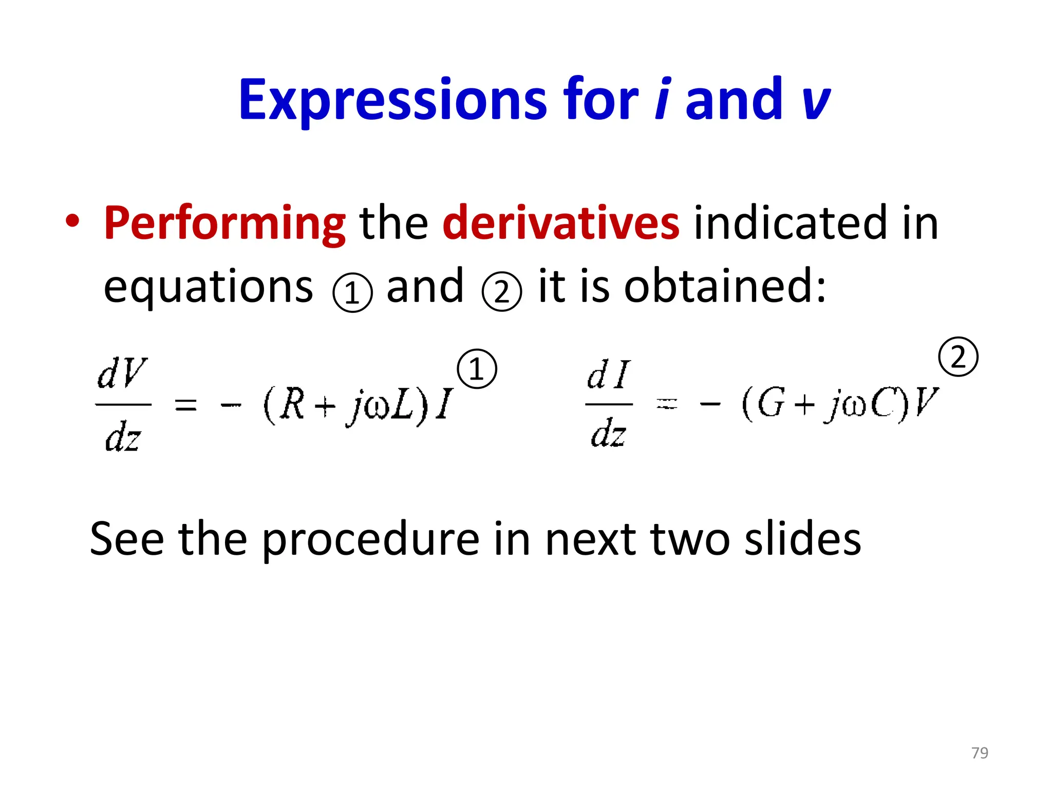
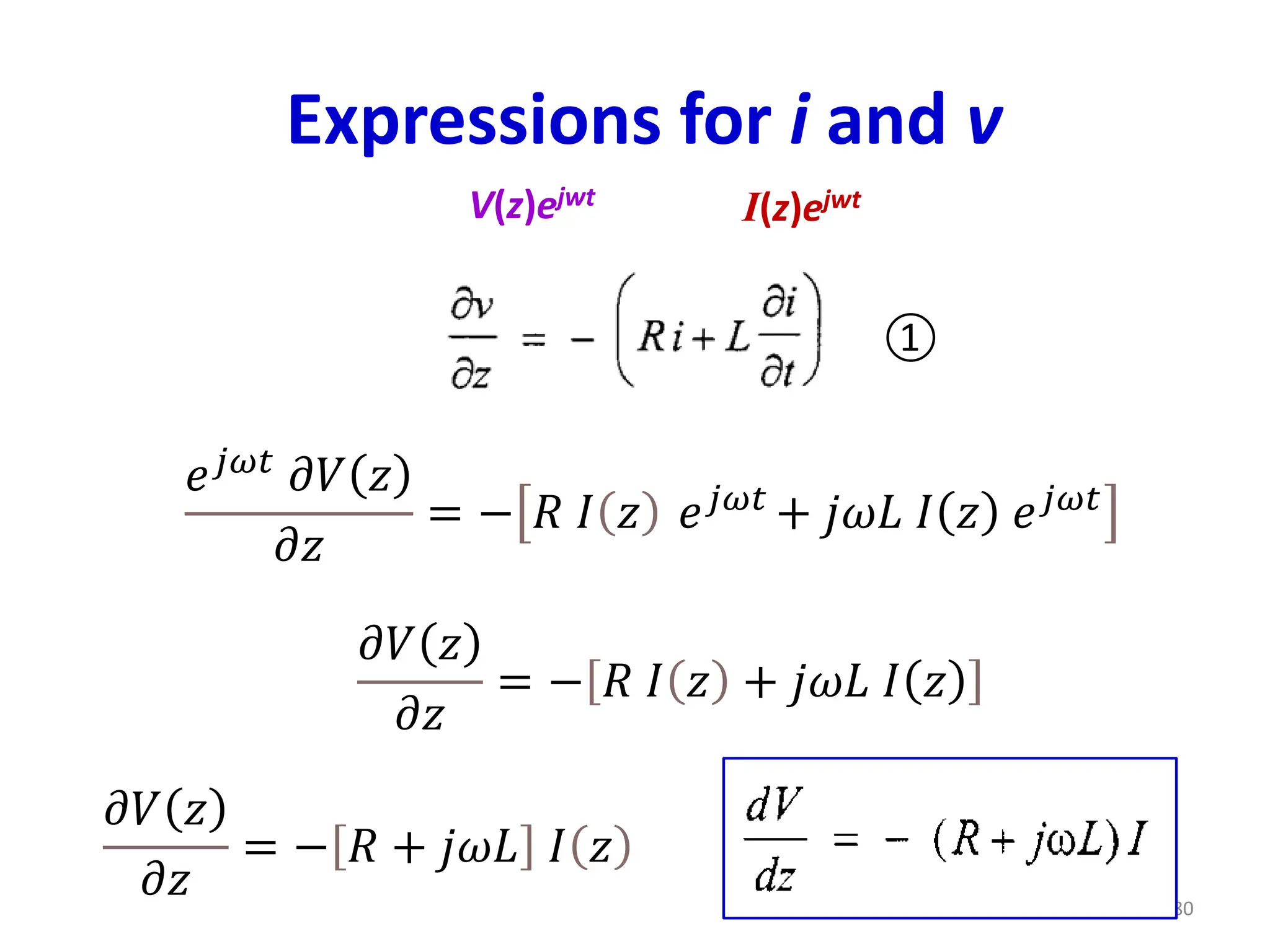
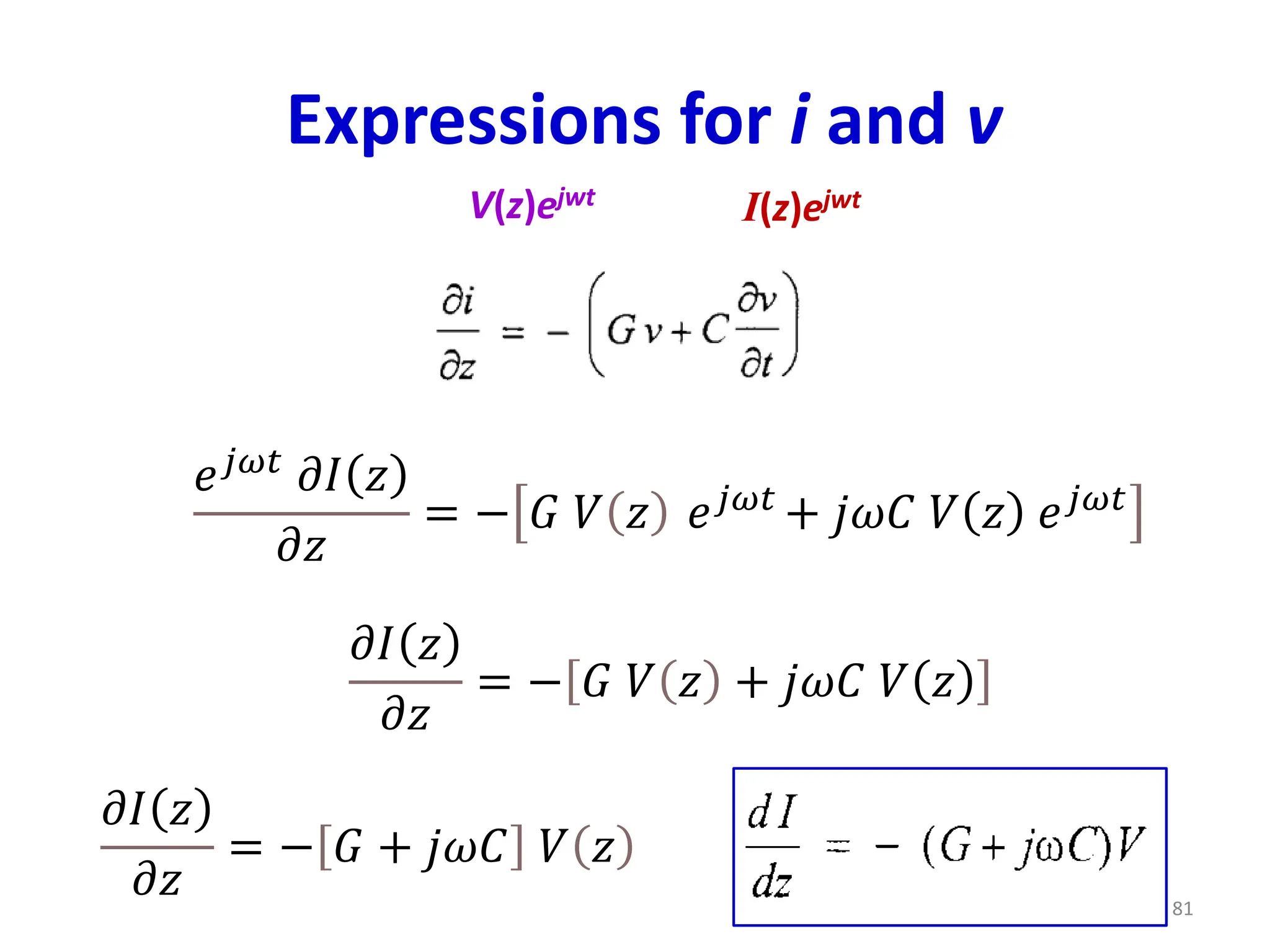
• Performing the derivatives indicated in
equations and it is obtained:
See the procedure in next two slides
79
① ②
① ②
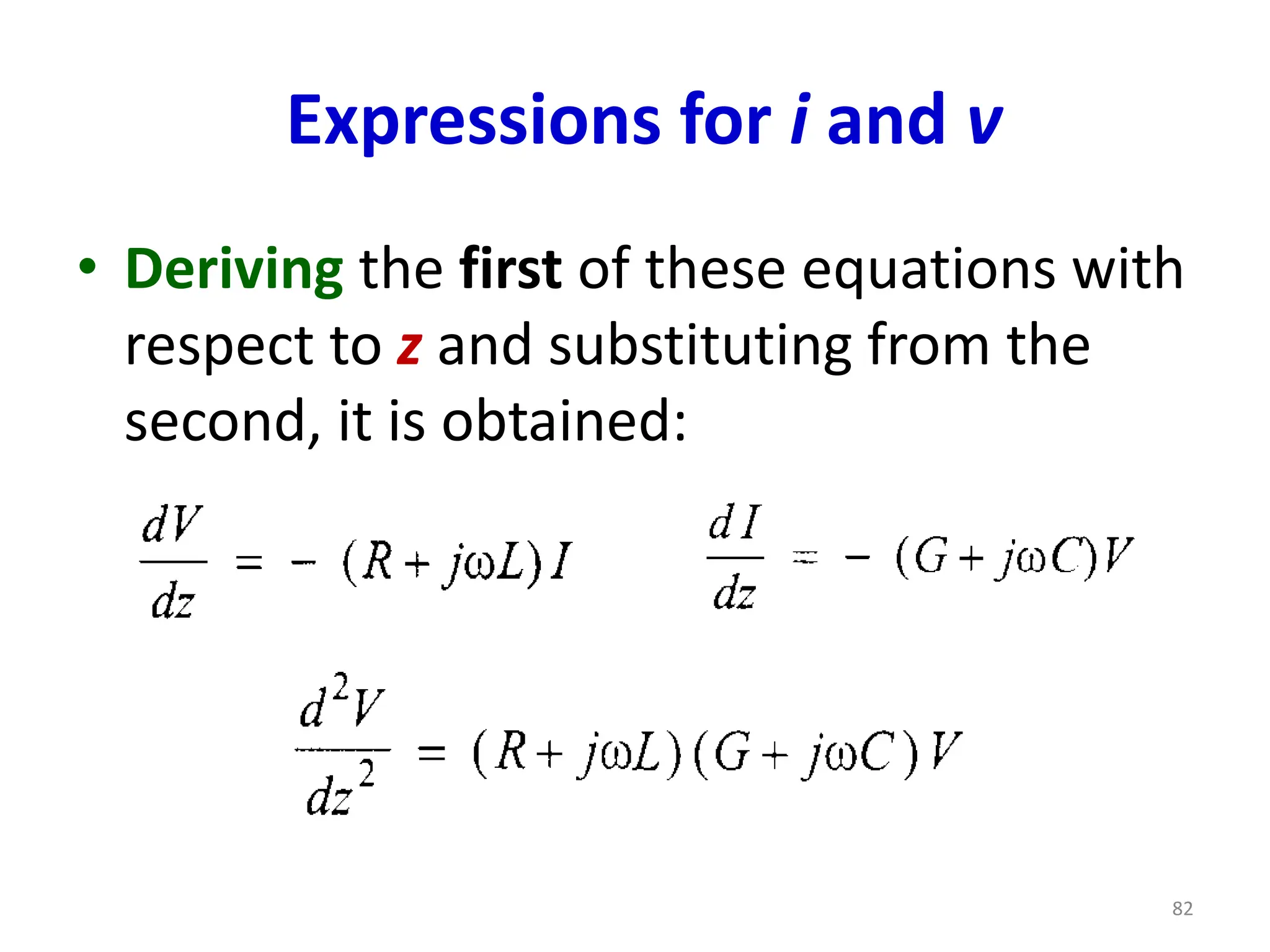
Expressions for iand v
• Deriving the first of these equations with
respect to z and substituting from the
second, it is obtained:
82
83.
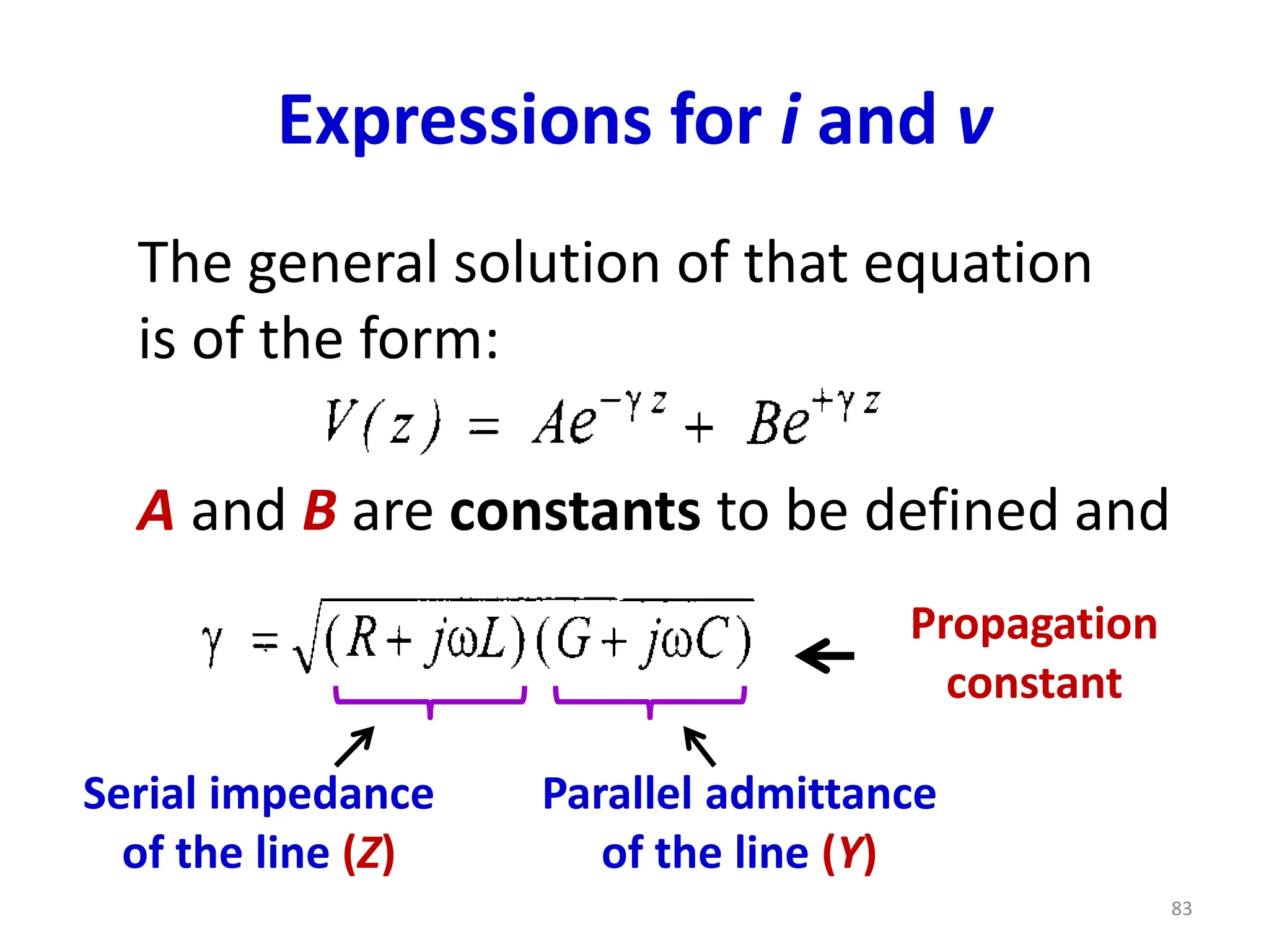
Expressions for iand v
The general solution of that equation
is of the form:
A and B are constants to be defined and
Propagation
constant
Serial impedance
of the line (Z)
Parallel admittance
of the line (Y)
83
84.
Expressions for iand v
• It has been seen that the parameters R,
L, G and C are not constant (they depend
on f).
• But if the line is uniform in its geometry
and composition of its materials along its
entire length (R, L, G and C independent
of z and t), they can be considered as
constant coefficients at a given
frequency. 84
85.
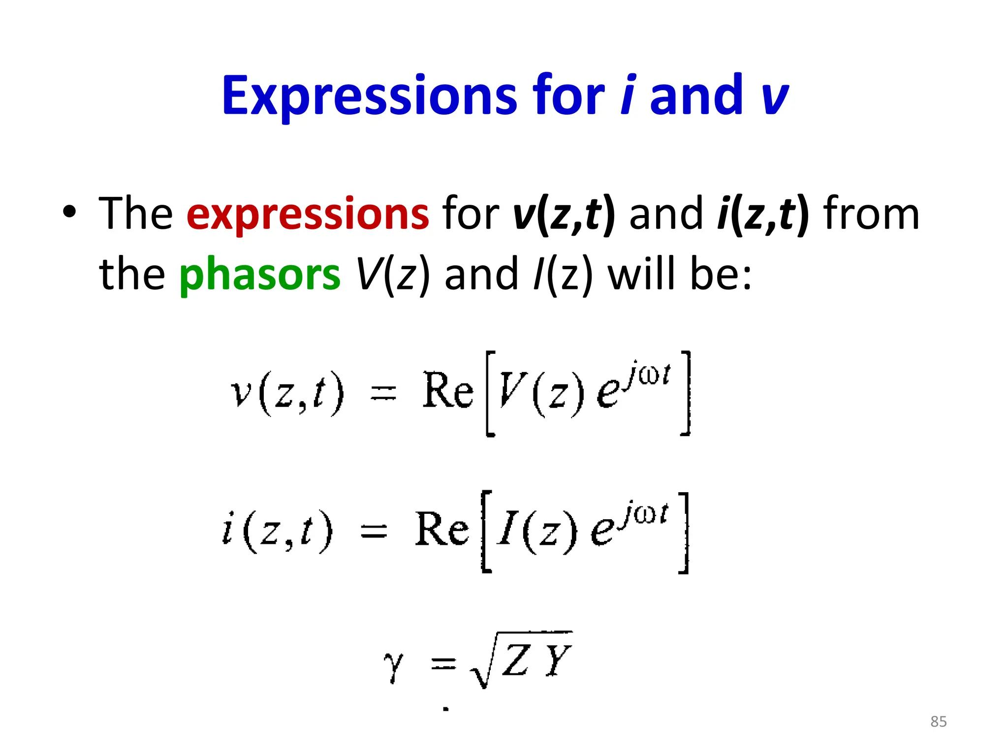
Expressions for iand v
• The expressions for v(z,t) and i(z,t) from
the phasors V(z) and I(z) will be:
85
86.
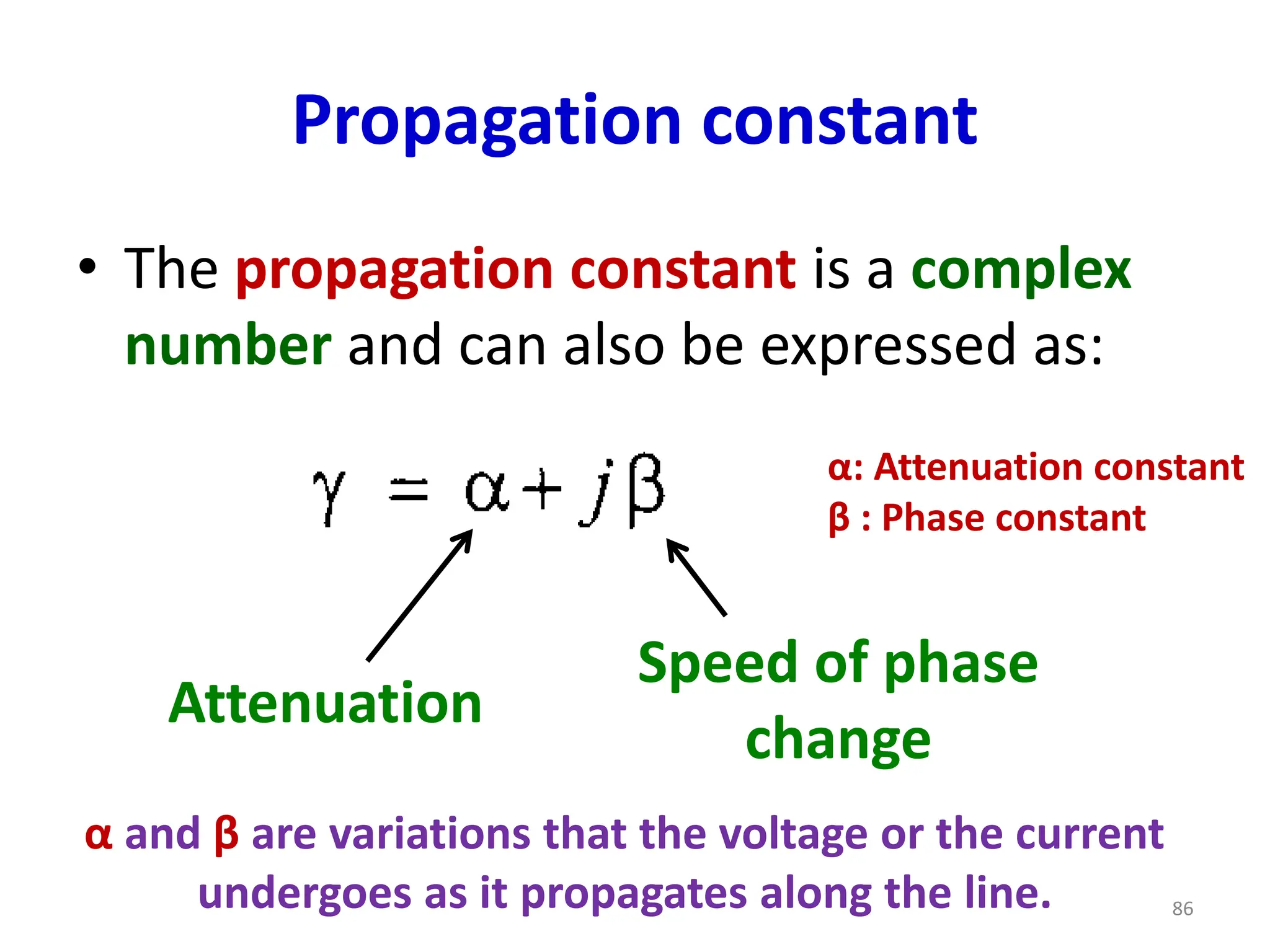
Propagation constant
• Thepropagation constant is a complex
number and can also be expressed as:
Attenuation
Speed of phase
change
α and β are variations that the voltage or the current
undergoes as it propagates along the line. 86
α: Attenuation constant
β : Phase constant
87.
Propagation constant
• Unitsof the attenuation constant α:
nepers per meter.
• Units of the phase constant β: radians
per meter.
• However, it is more common to specify α
in decibels per meter and use the letter L
(Loss).
87
88.
Propagation constant
• Theconversion from nepers to decibels
can be done using the following ratio:
• Attenuation:
L (dB/m) = 8.686 x α (Np/m)
1 neper equal to 8.686 dB.
88
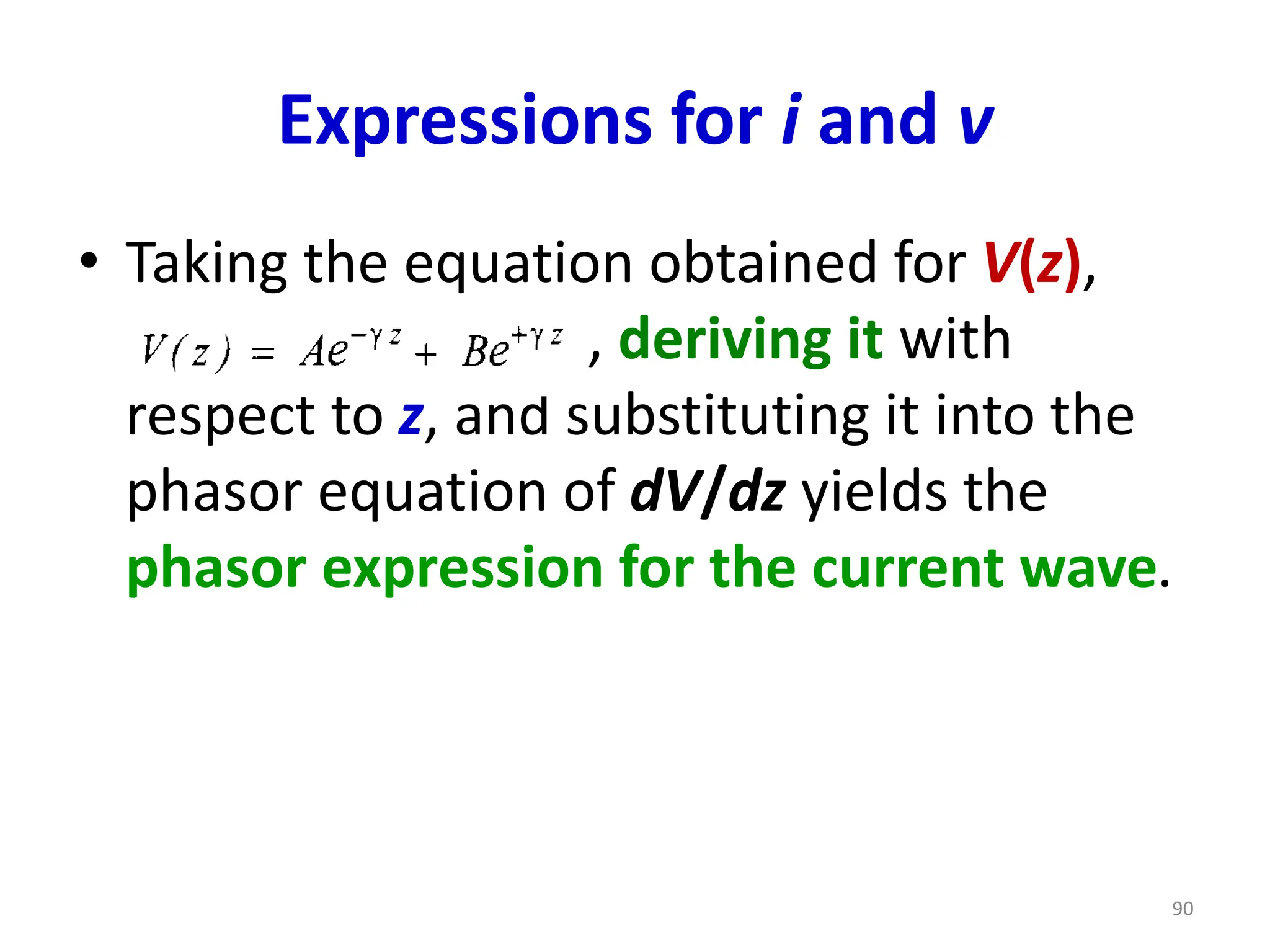
Expressions for iand v
• Taking the equation obtained for V(z),
, deriving it with
respect to z, and substituting it into the
phasor equation of dV/dz yields the
phasor expression for the current wave.
90
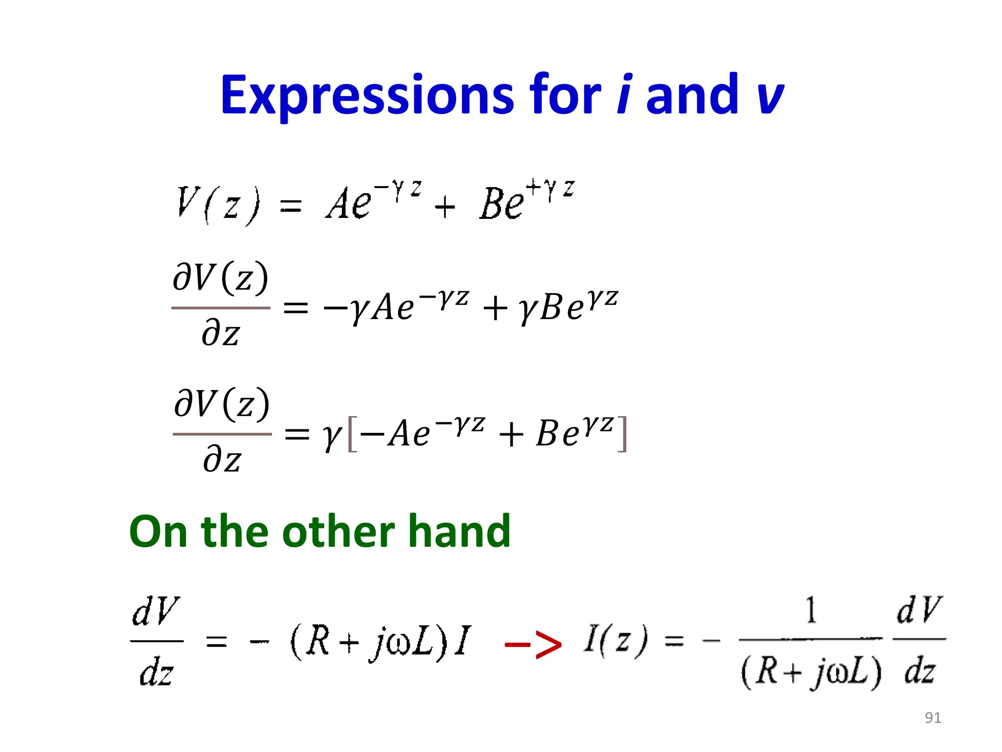
91.
Expressions for iand v
91
𝜕𝑉 𝑧
𝜕𝑧
= −𝛾𝐴𝑒−𝛾𝑧 + 𝛾𝐵𝑒𝛾𝑧
𝜕𝑉 𝑧
𝜕𝑧
= 𝛾 −𝐴𝑒−𝛾𝑧
+ 𝐵𝑒𝛾𝑧
−>
On the other hand
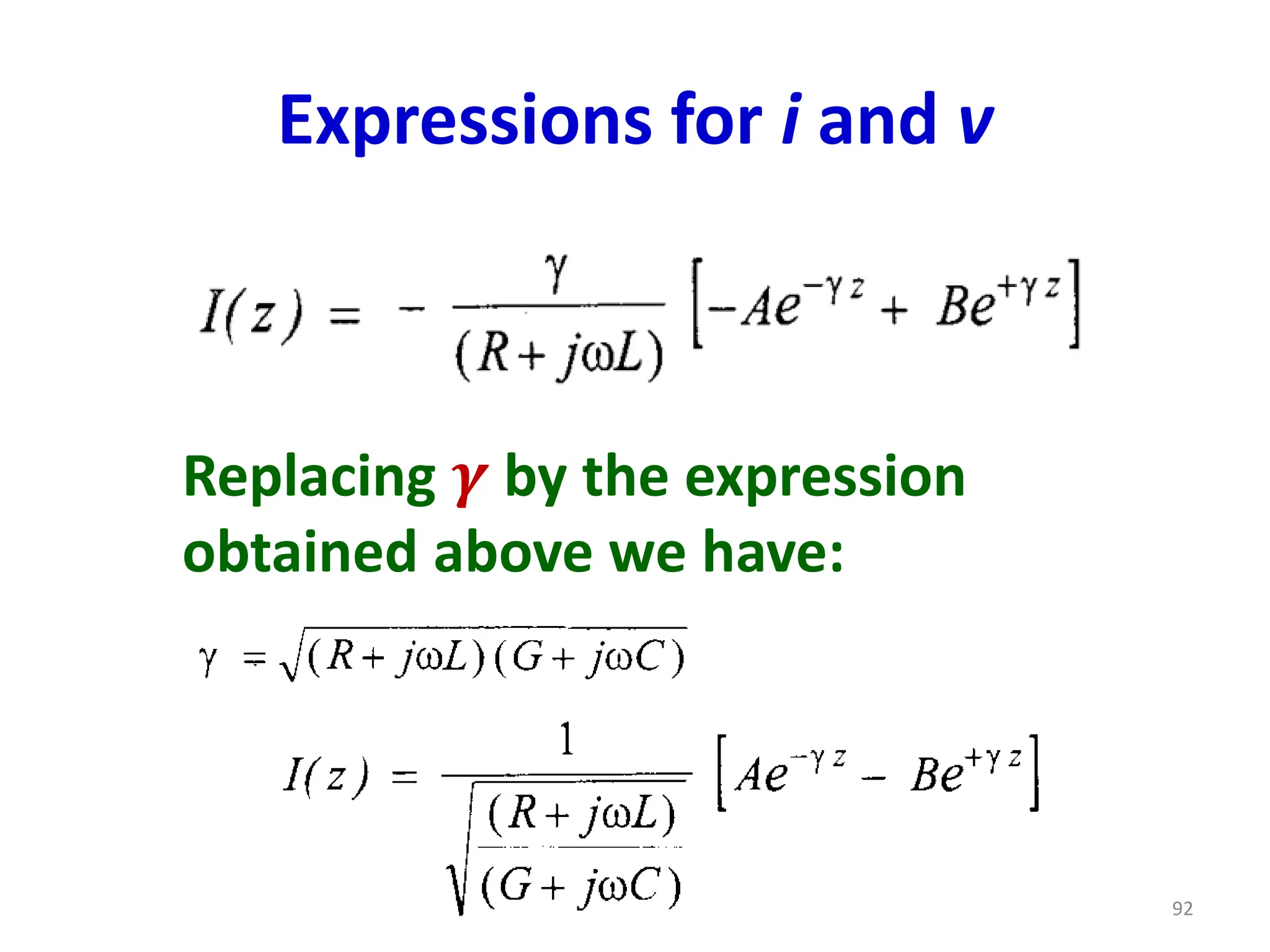
92.
Expressions for iand v
92
Replacing 𝜸 by the expression
obtained above we have:
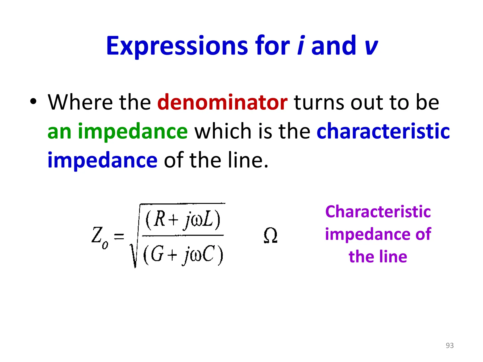
93.
Expressions for iand v
• Where the denominator turns out to be
an impedance which is the characteristic
impedance of the line.
Characteristic
impedance of
the line
93
94.
Characteristic impedance Z0
•Every transmission line has its own
characteristic impedance Z0, depending
on the geometry and dimensions of the
line, as well as the operating frequency f
(ω = 2πf).
• Z0 is commonly provided by cable
manufacturers.
ω = Angular frequency 94
95.
Characteristic impedance Z0
•There are cables with nominal
characteristic impedances such as:
–Coaxial for broadcasting and computers: 50
Ω.
–Coaxial for CATV: 75 Ω.
–Two-wire cables: 300 Ω (Rx TV or FM
antennas)
–Multipair bi-wire cables for telephony and
data: 75 Ω, 100 Ω, 150 Ω, 600 Ω, etc.
95
96.
Characteristic impedance Z0
•So far, two new transmission line
parameters have been defined:
–Propagation constant (γ)
–Characteristic impedance (Z0).
• Z0 and γ are complex numbers and they
are a function of f and of the basic
parameters R, L, G and C.
96
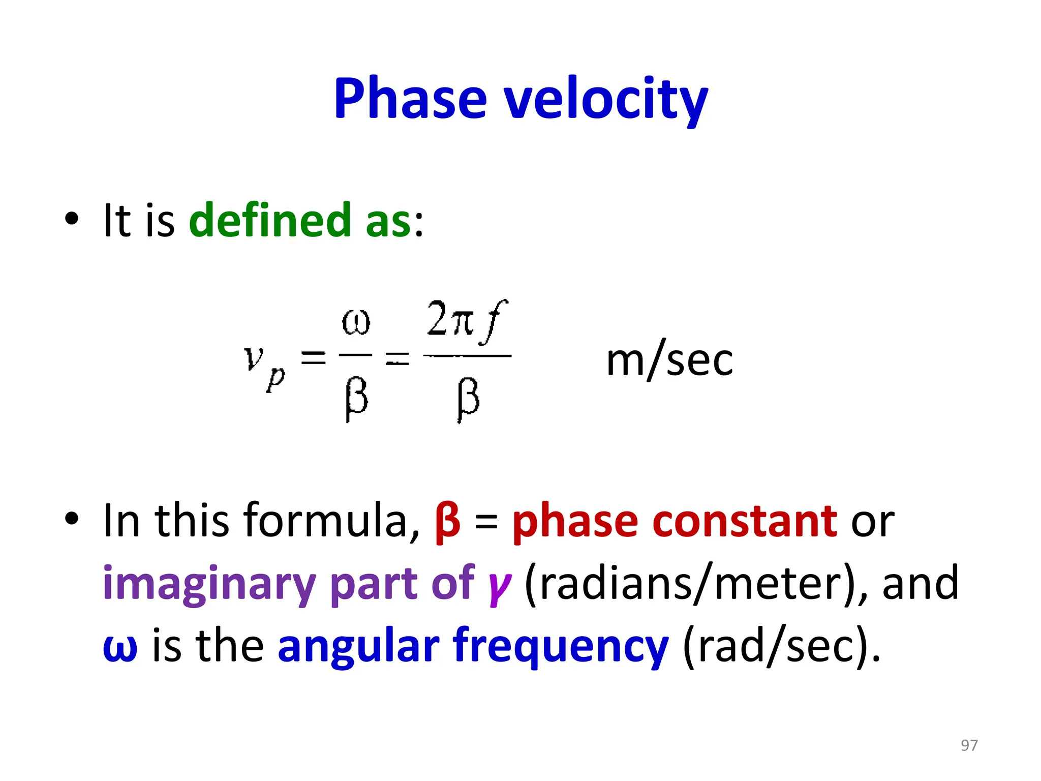
97.
Phase velocity
• Itis defined as:
• In this formula, β = phase constant or
imaginary part of γ (radians/meter), and
ω is the angular frequency (rad/sec).
97
m/sec
98.
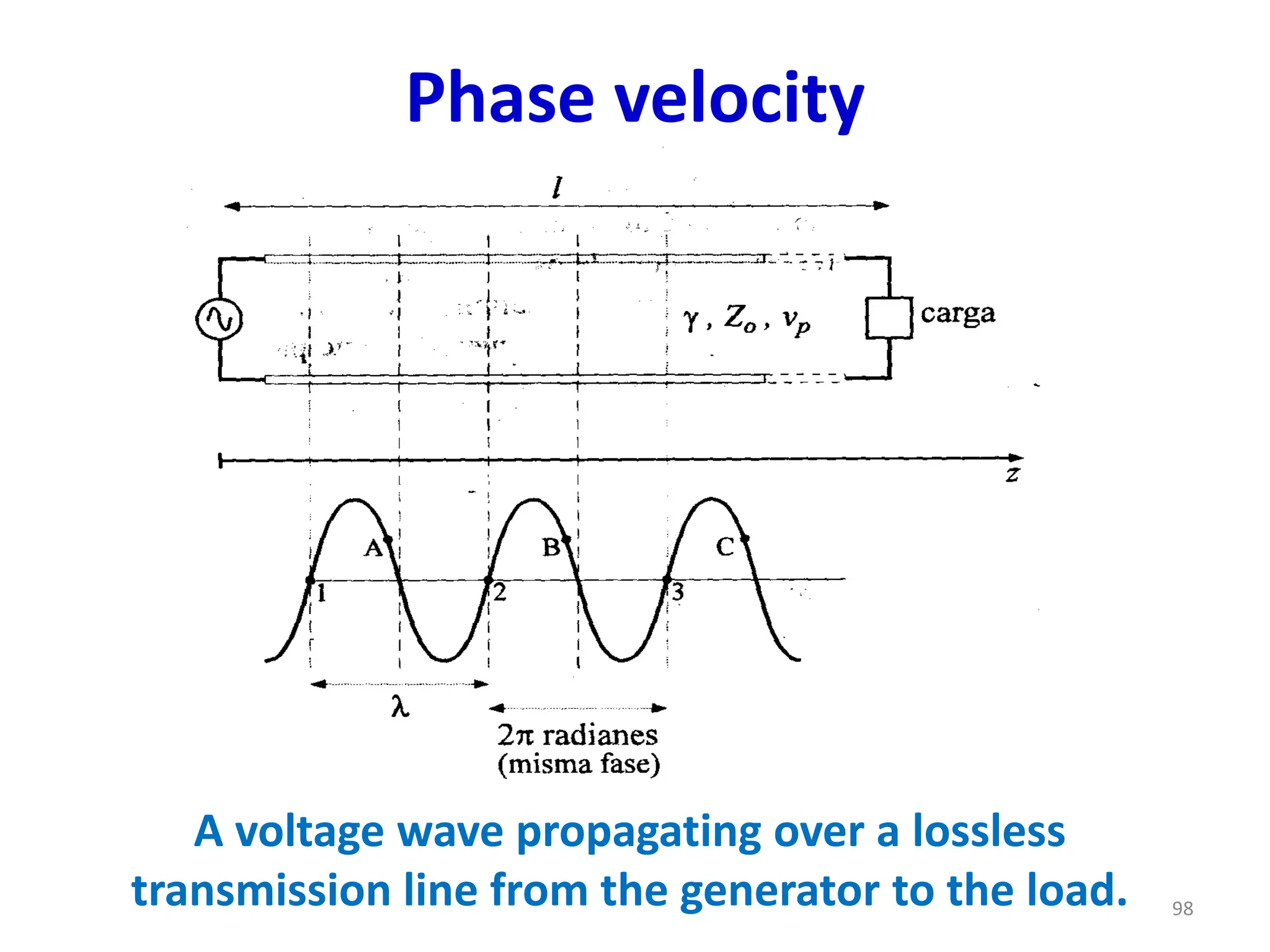
Phase velocity
A voltagewave propagating over a lossless
transmission line from the generator to the load. 98
99.
Phase velocity
• Aline with no attenuation is assumed (α =
0), that is, the wave is not damped (γ is
purely imaginary).
• The line has a physical length given in
meters and an electrical length measured
in λs.
• λ: distance between successive points of
the wave with the same electrical phase.
99
100.
Propagation velocity
• Thevalue of λ depends on the frequency
(f) of oscillation and the propagation
velocity (v).
• This velocity, in turn, depends on the
characteristics of the medium through
which the wave travels (type of dielectric
between the conductors of the line).
100
101.
Propagation velocity
• Ifthere is air between the conductors,
the v of the wave is equal to that of the
light in free space (3x10⁸ m/sec).
• But if the medium has a relative
dielectric constant εr > 1, then the wave
propagates with a speed less than the
light velocity.
101
102.
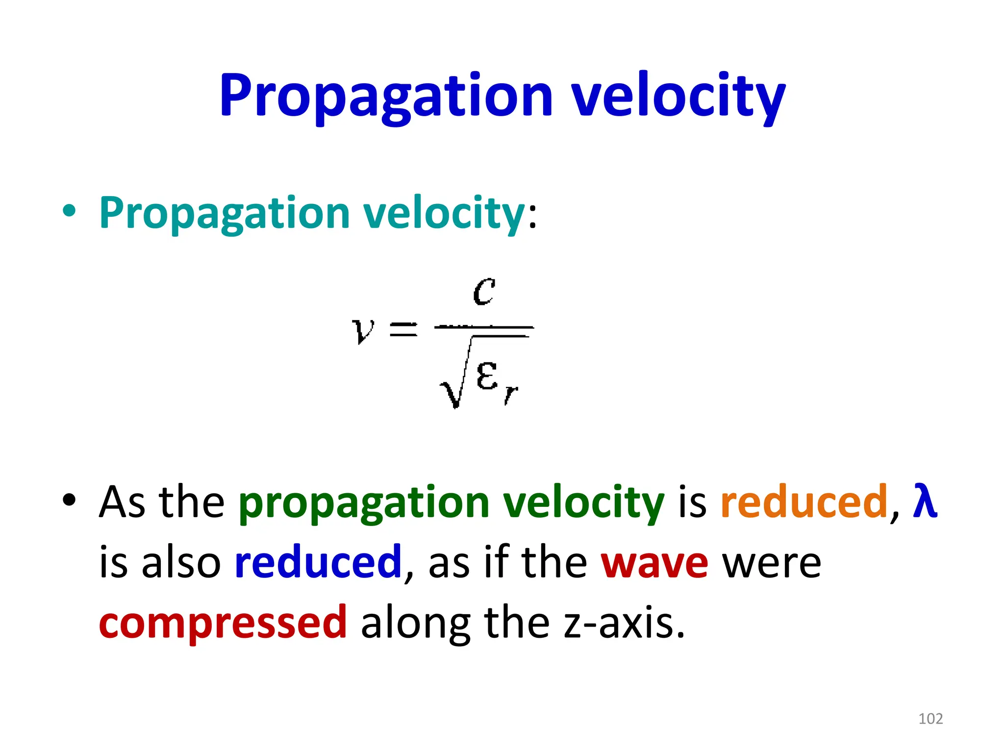
Propagation velocity
• Propagationvelocity:
• As the propagation velocity is reduced, λ
is also reduced, as if the wave were
compressed along the z-axis.
102
103.
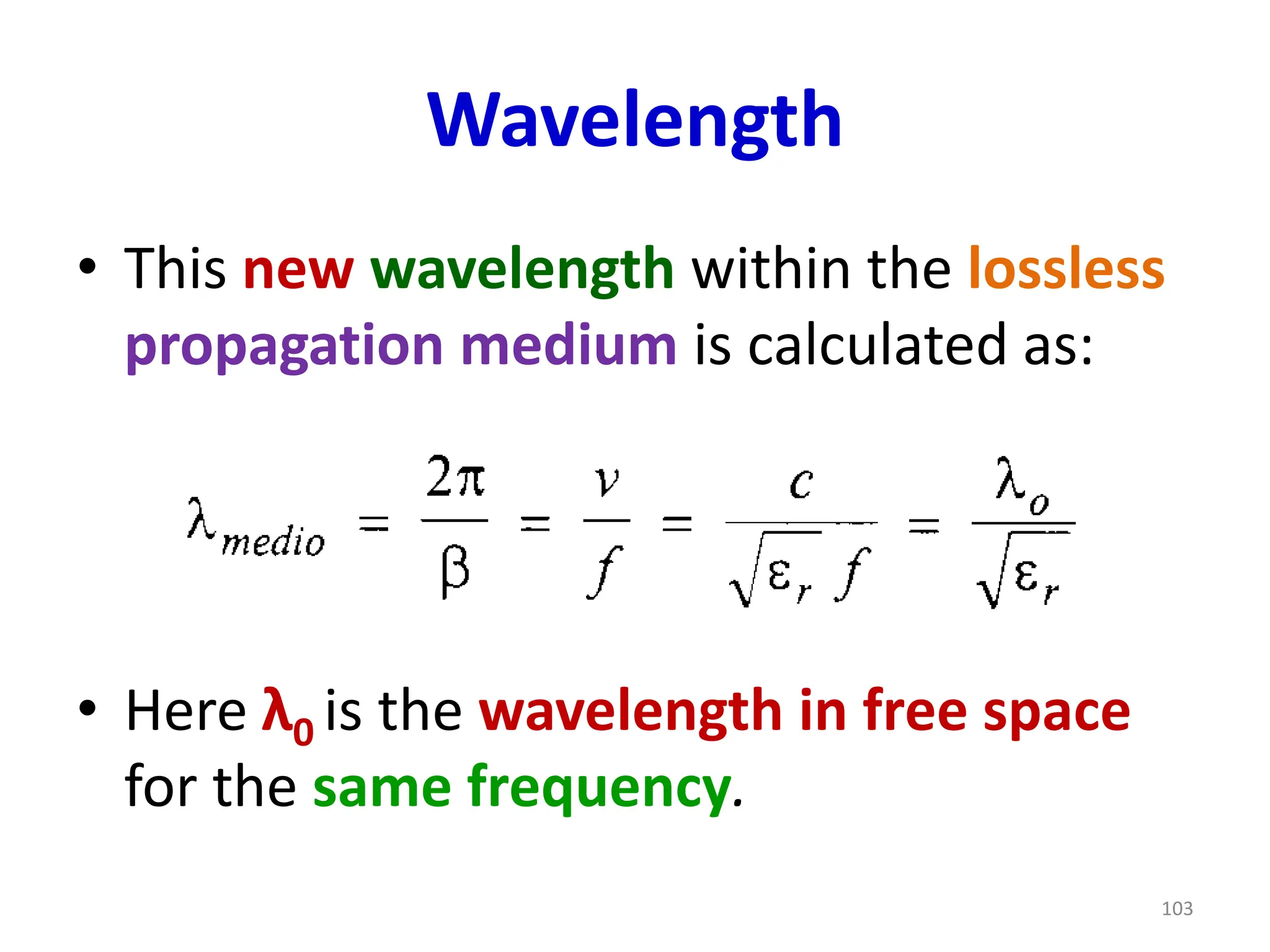
Wavelength
• This newwavelength within the lossless
propagation medium is calculated as:
• Here λ0 is the wavelength in free space
for the same frequency.
103
104.
Phase velocity
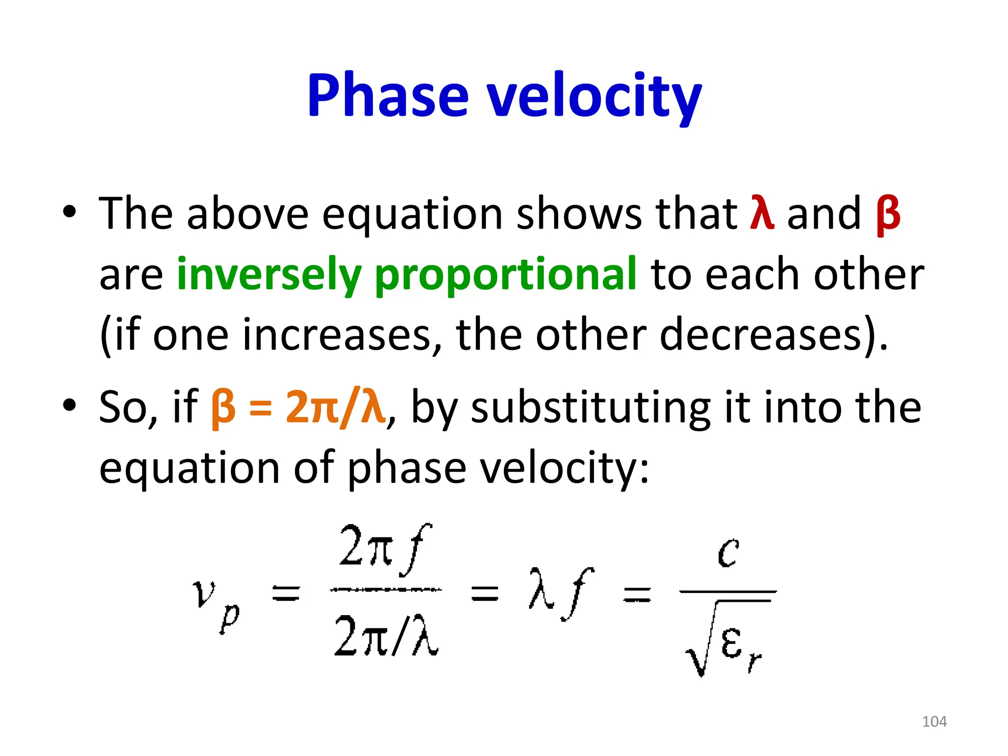
• Theabove equation shows that λ and β
are inversely proportional to each other
(if one increases, the other decreases).
• So, if β = 2π/λ, by substituting it into the
equation of phase velocity:
104
105.
Phase velocity
• vpis independent of f (if the medium is
considered lossless, α = 0) and is the
speed with which moves a point, say B,
that defines the location of a given
constant phase.
• In other words, vp is the speed at which
an imaginary point, at which the phase is
constant, moves in the direction of z.
105
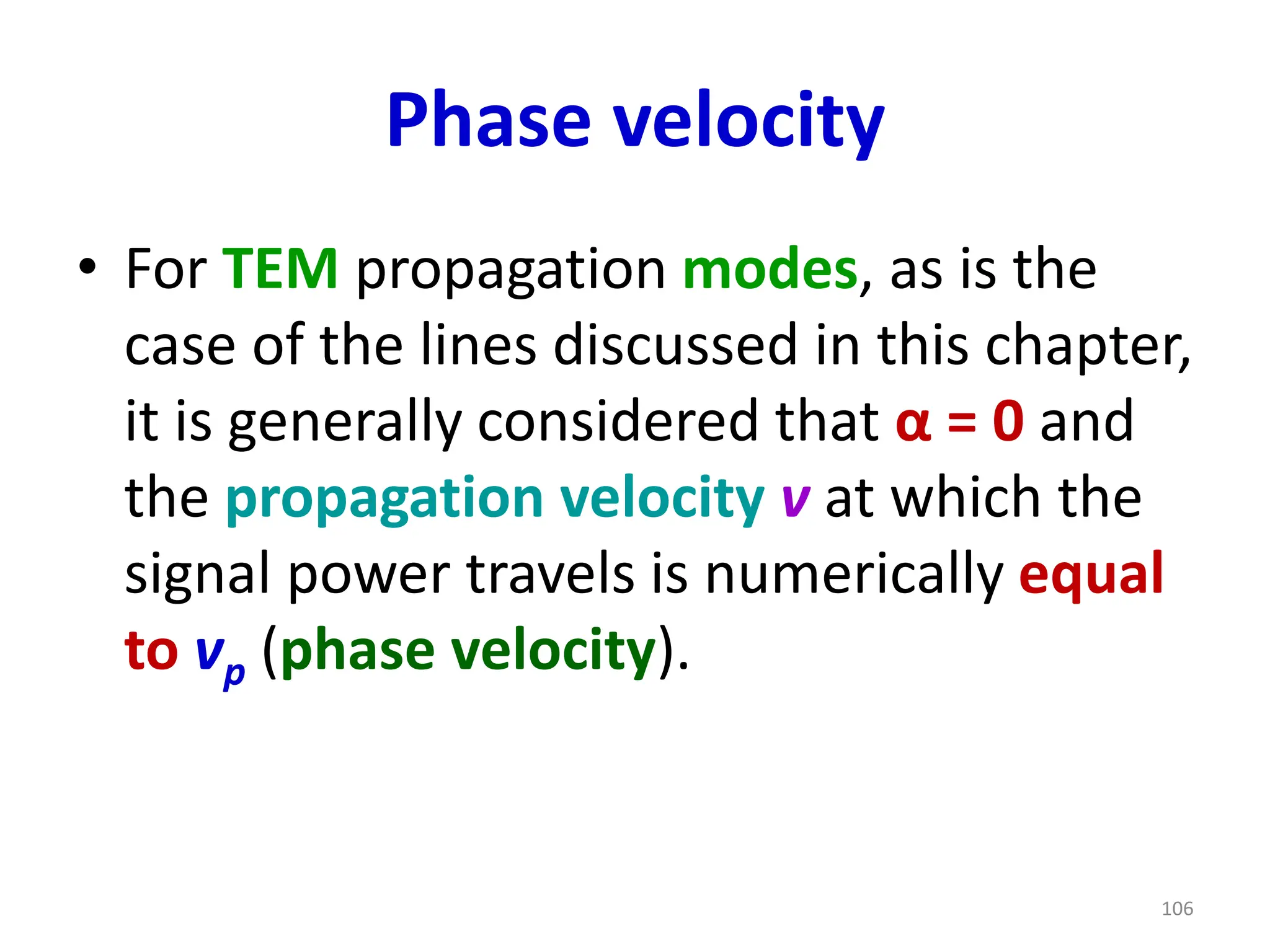
106.
Phase velocity
• ForTEM propagation modes, as is the
case of the lines discussed in this chapter,
it is generally considered that α = 0 and
the propagation velocity v at which the
signal power travels is numerically equal
to vp (phase velocity).
106
107.
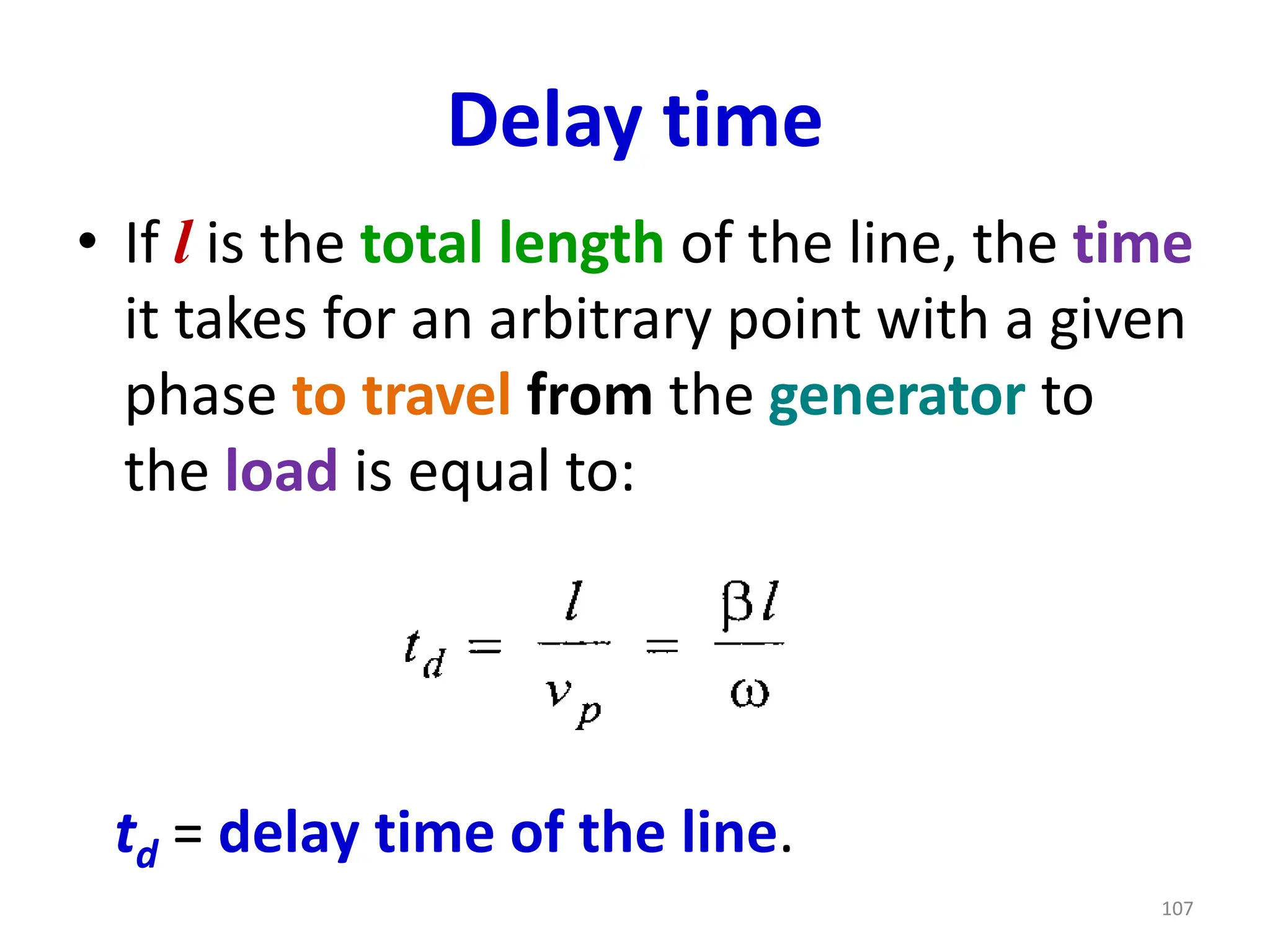
Delay time
• Ifl is the total length of the line, the time
it takes for an arbitrary point with a given
phase to travel from the generator to
the load is equal to:
td = delay time of the line.
107
108.
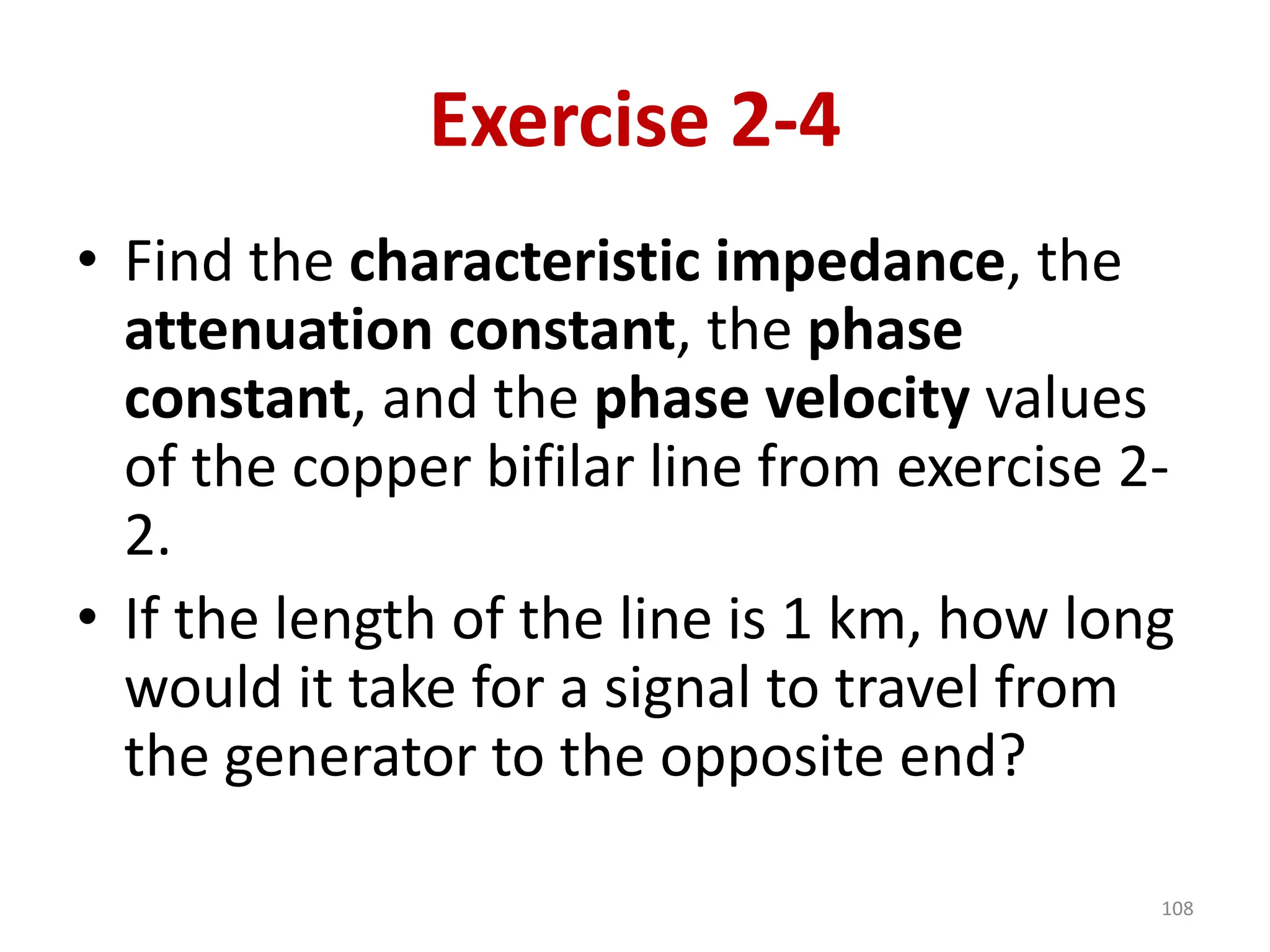
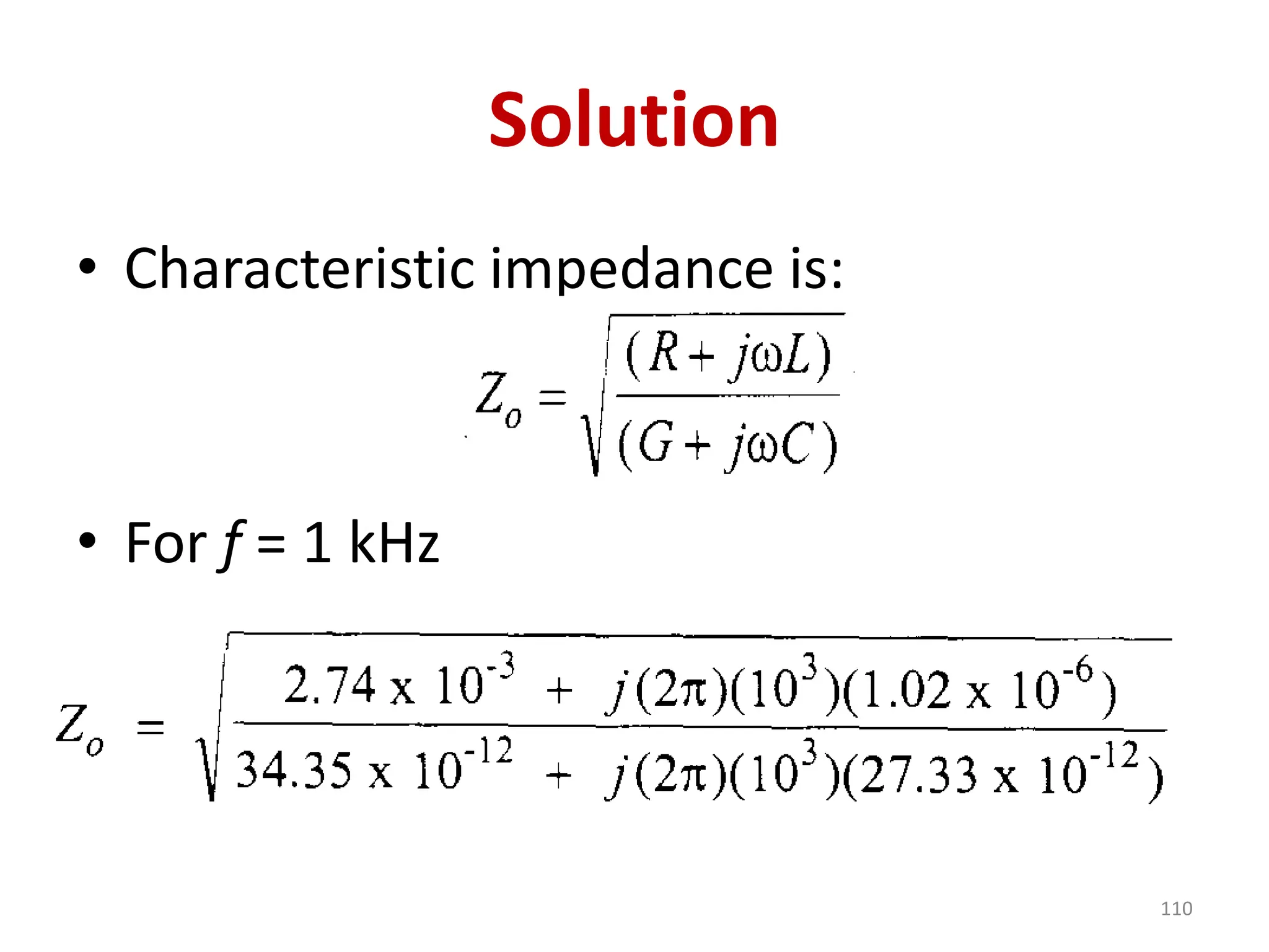
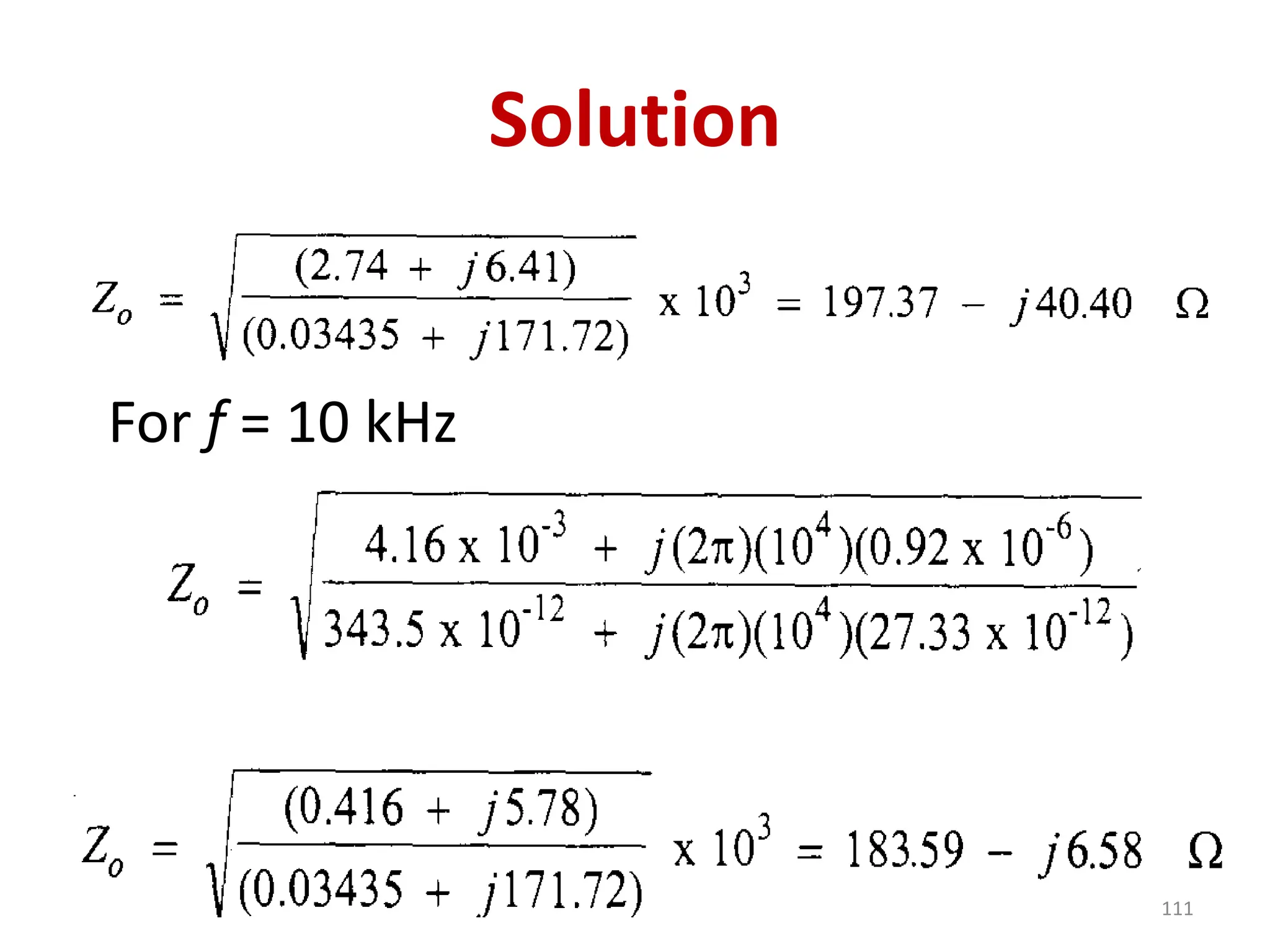
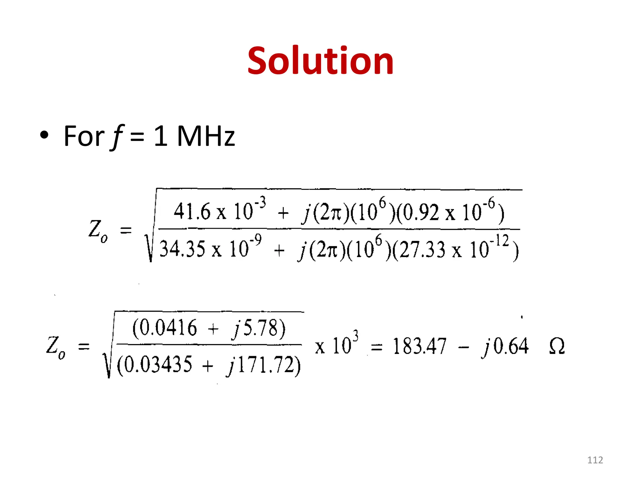
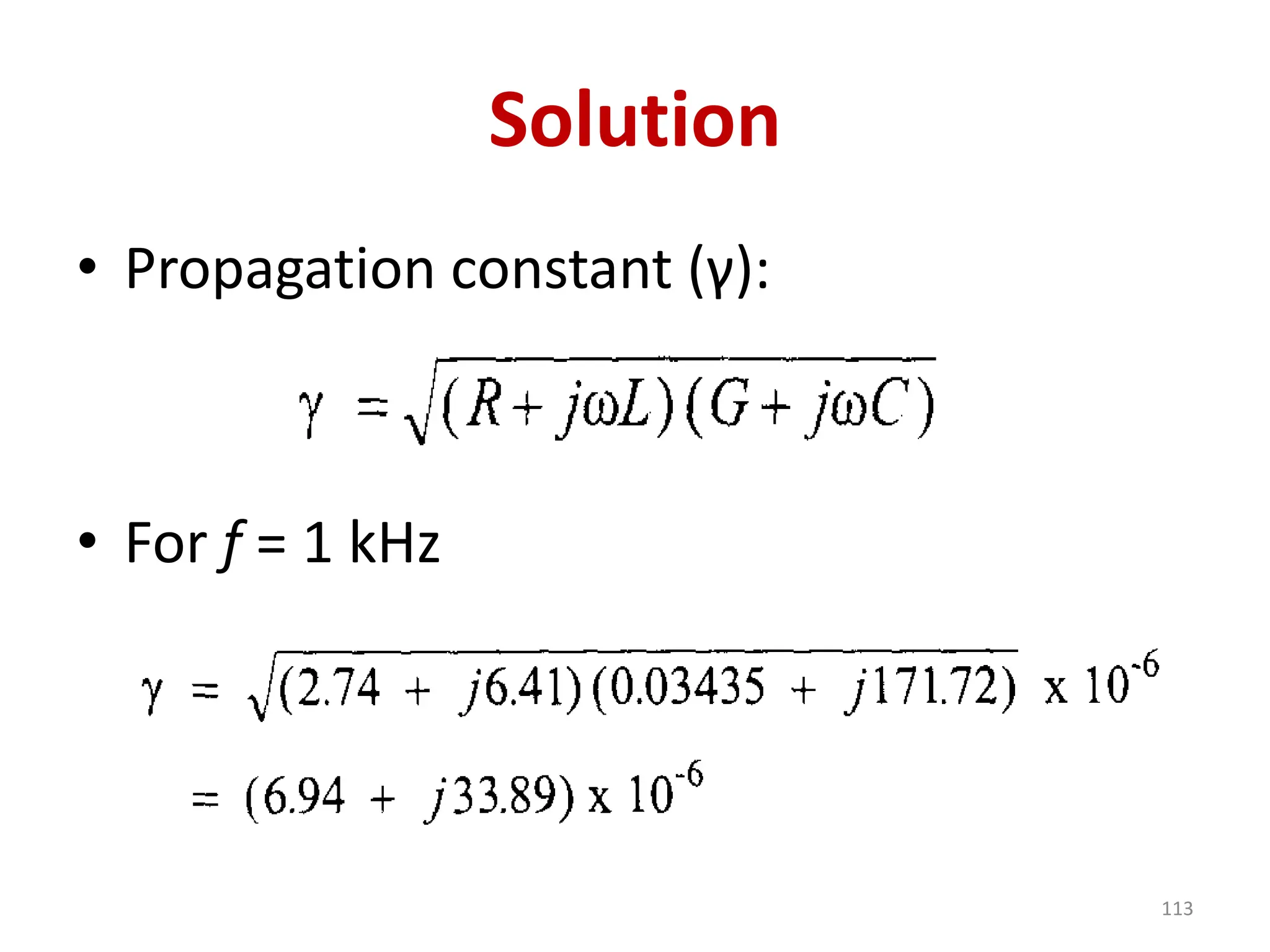
Exercise 2-4
• Findthe characteristic impedance, the
attenuation constant, the phase
constant, and the phase velocity values
of the copper bifilar line from exercise 2-
2.
• If the length of the line is 1 km, how long
would it take for a signal to travel from
the generator to the opposite end?
108
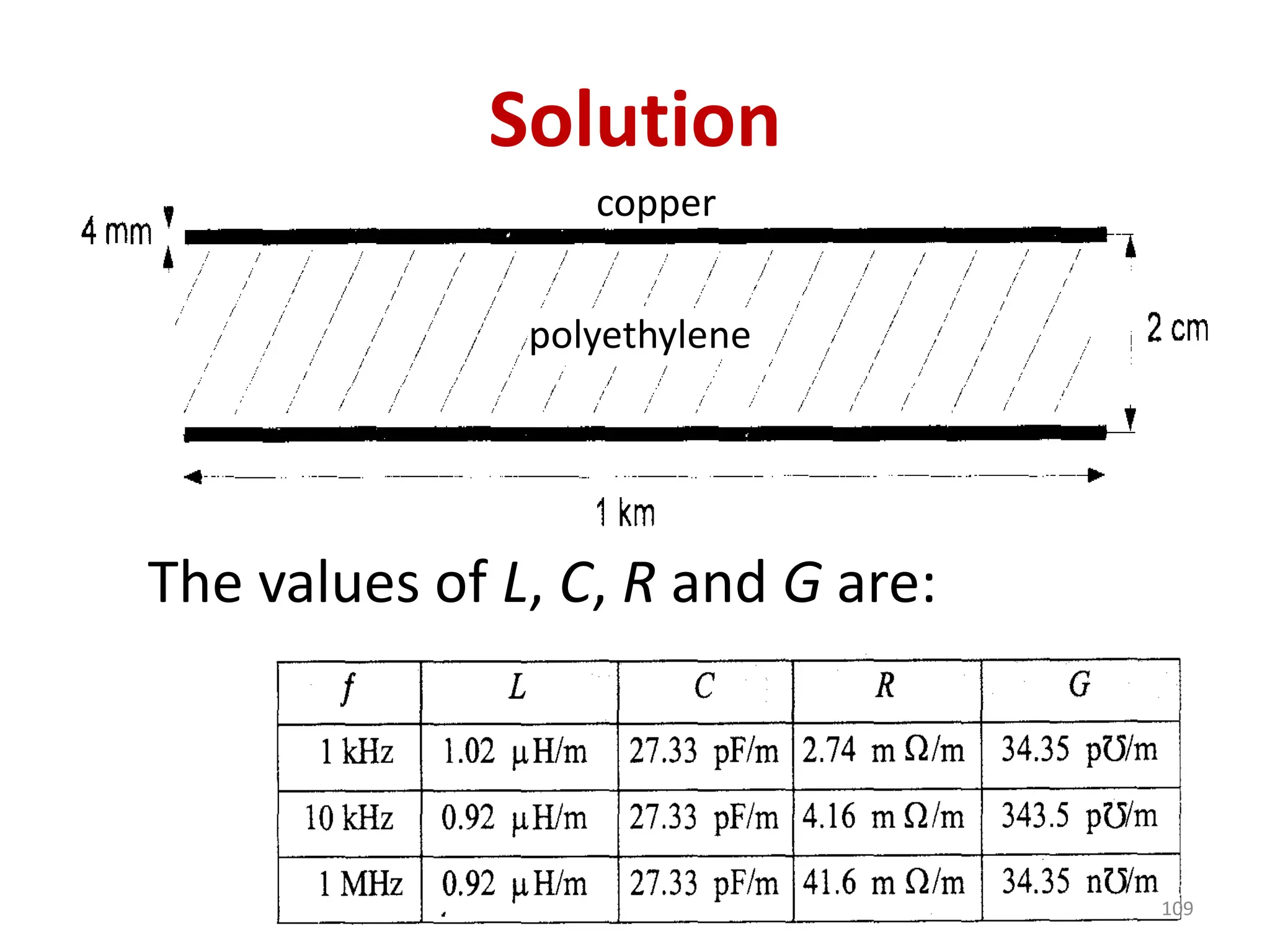
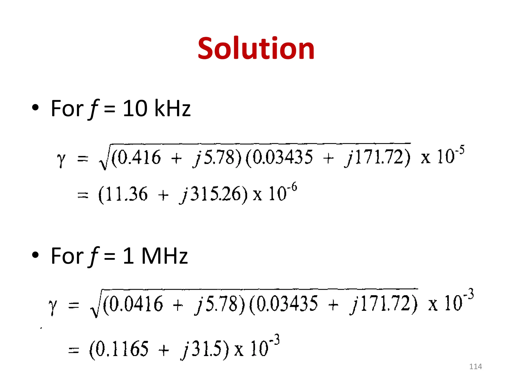
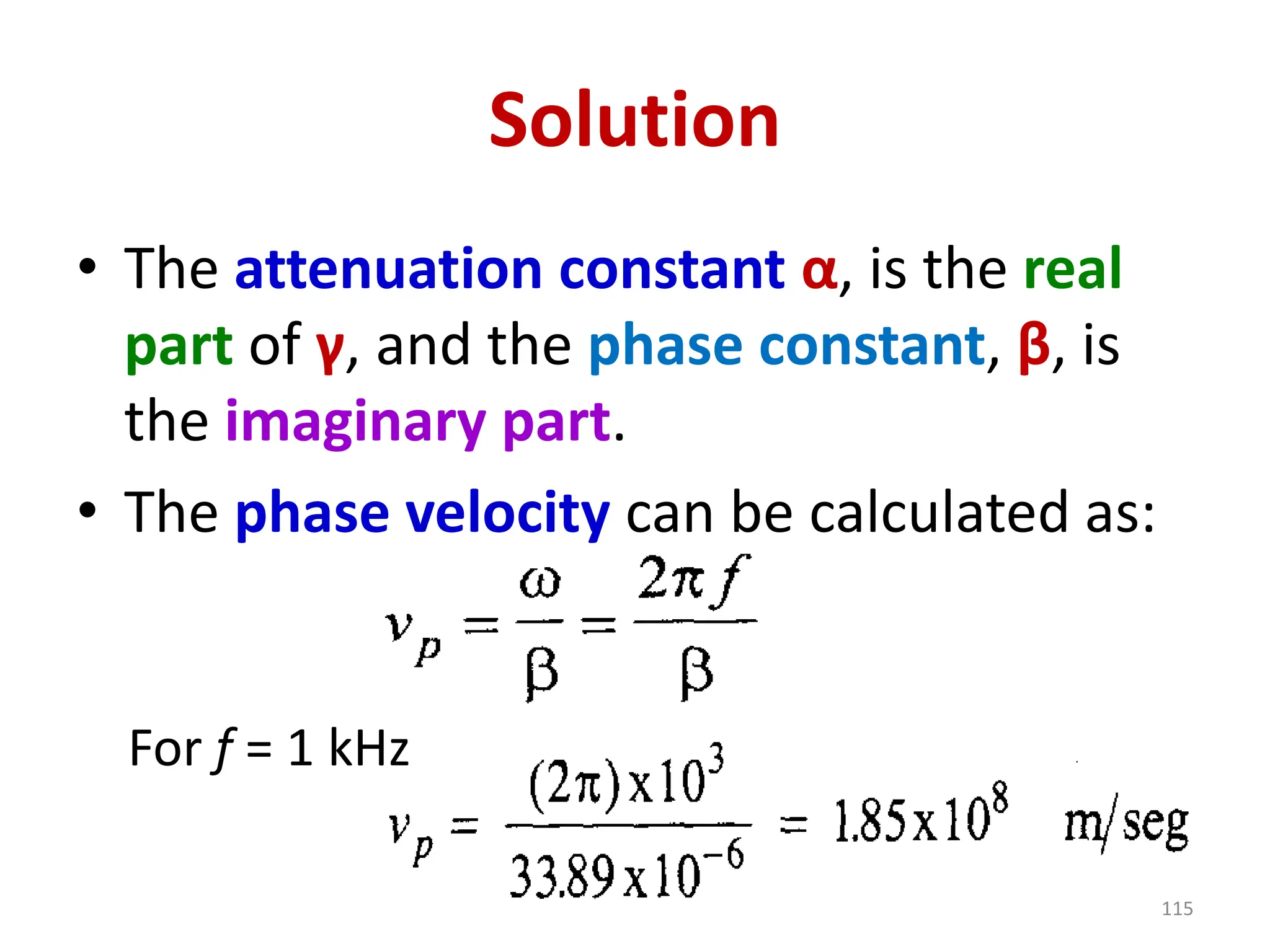
Solution
• The attenuationconstant α, is the real
part of γ, and the phase constant, β, is
the imaginary part.
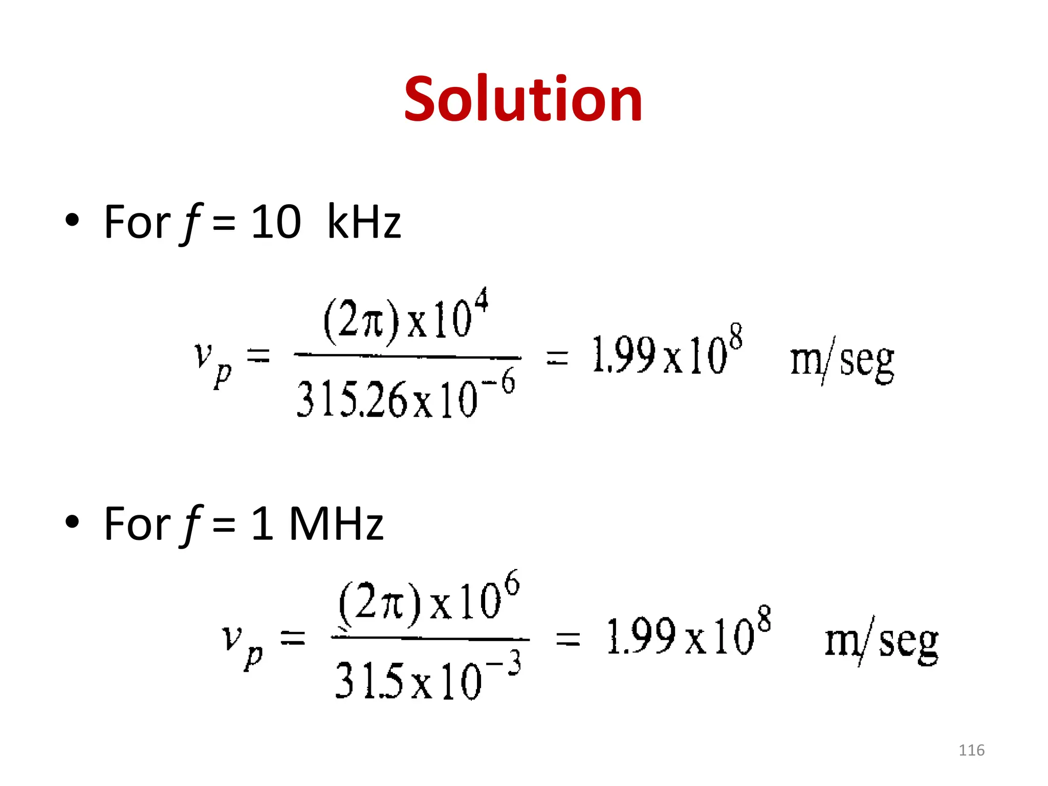
• The phase velocity can be calculated as:
For f = 1 kHz
115
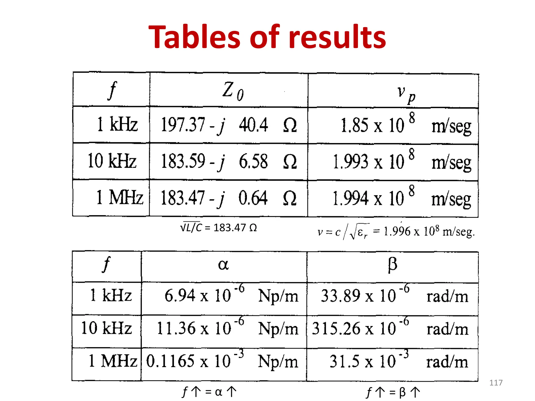
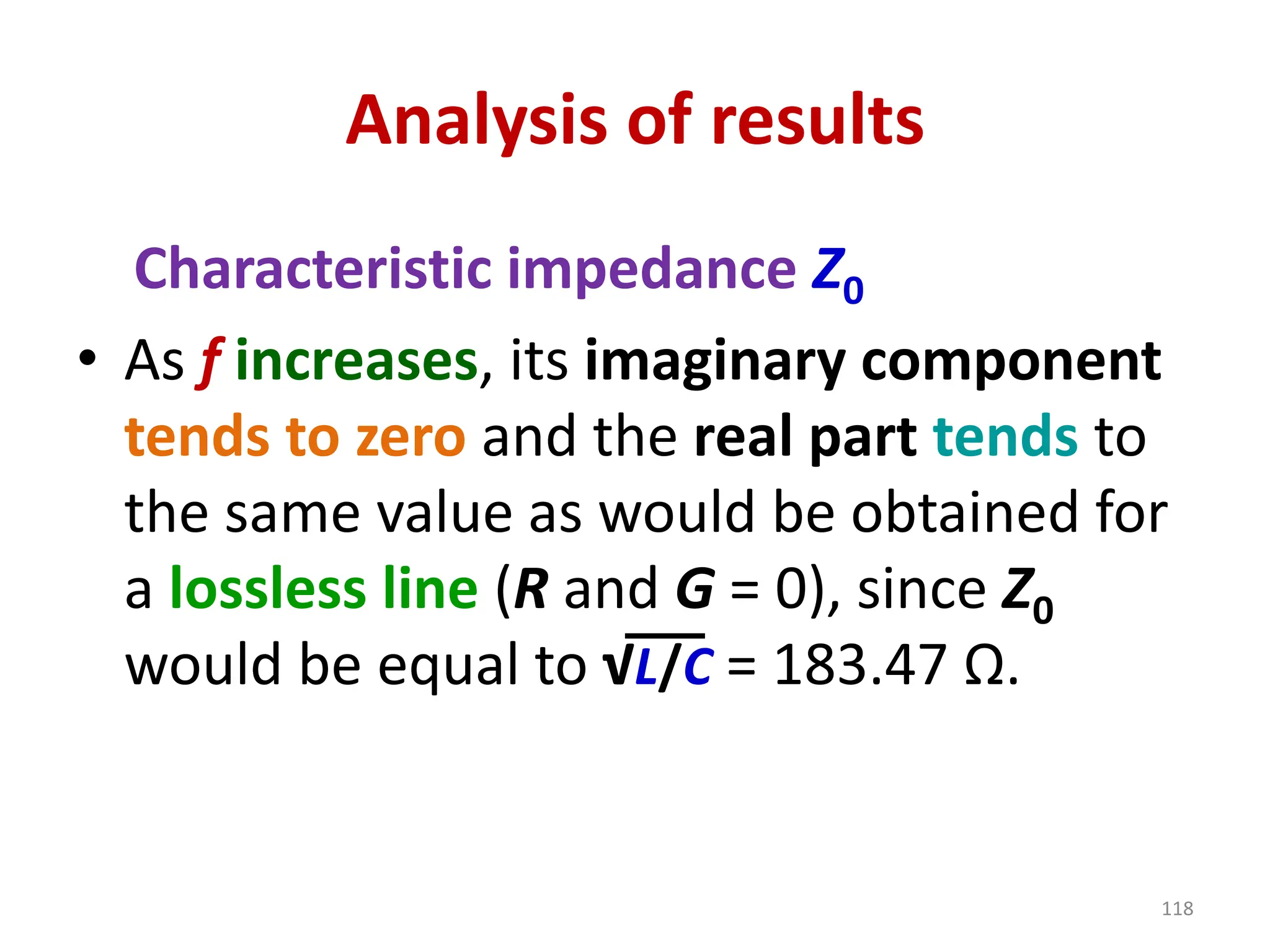
Analysis of results
Characteristicimpedance Z0
• As f increases, its imaginary component
tends to zero and the real part tends to
the same value as would be obtained for
a lossless line (R and G = 0), since Z0
would be equal to √L/C = 183.47 Ω.
118
119.
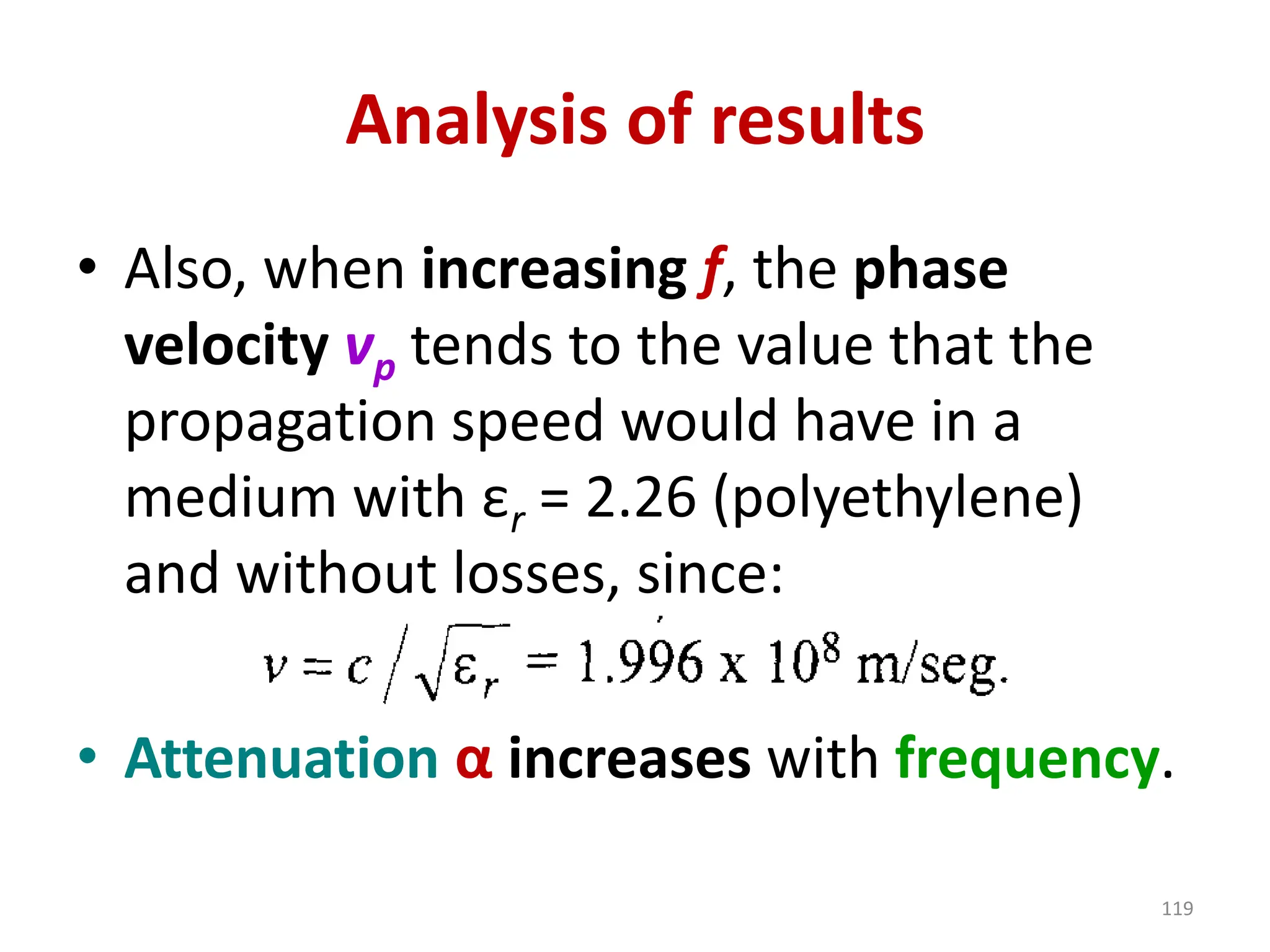
Analysis of results
•Also, when increasing f, the phase
velocity vp tends to the value that the
propagation speed would have in a
medium with εr = 2.26 (polyethylene)
and without losses, since:
• Attenuation α increases with frequency.
119
120.
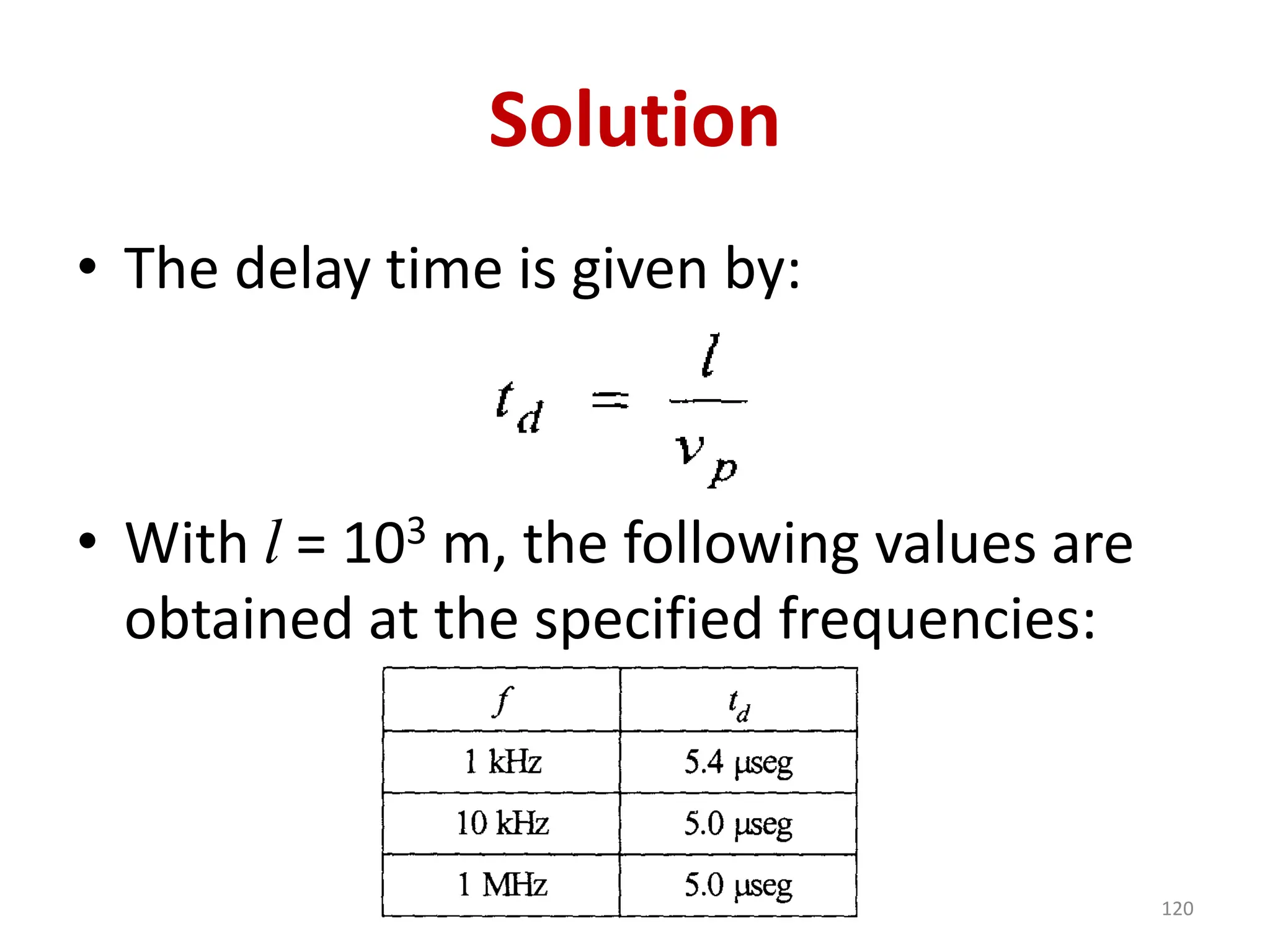
Solution
• The delaytime is given by:
• With l = 103 m, the following values are
obtained at the specified frequencies:
120
121.
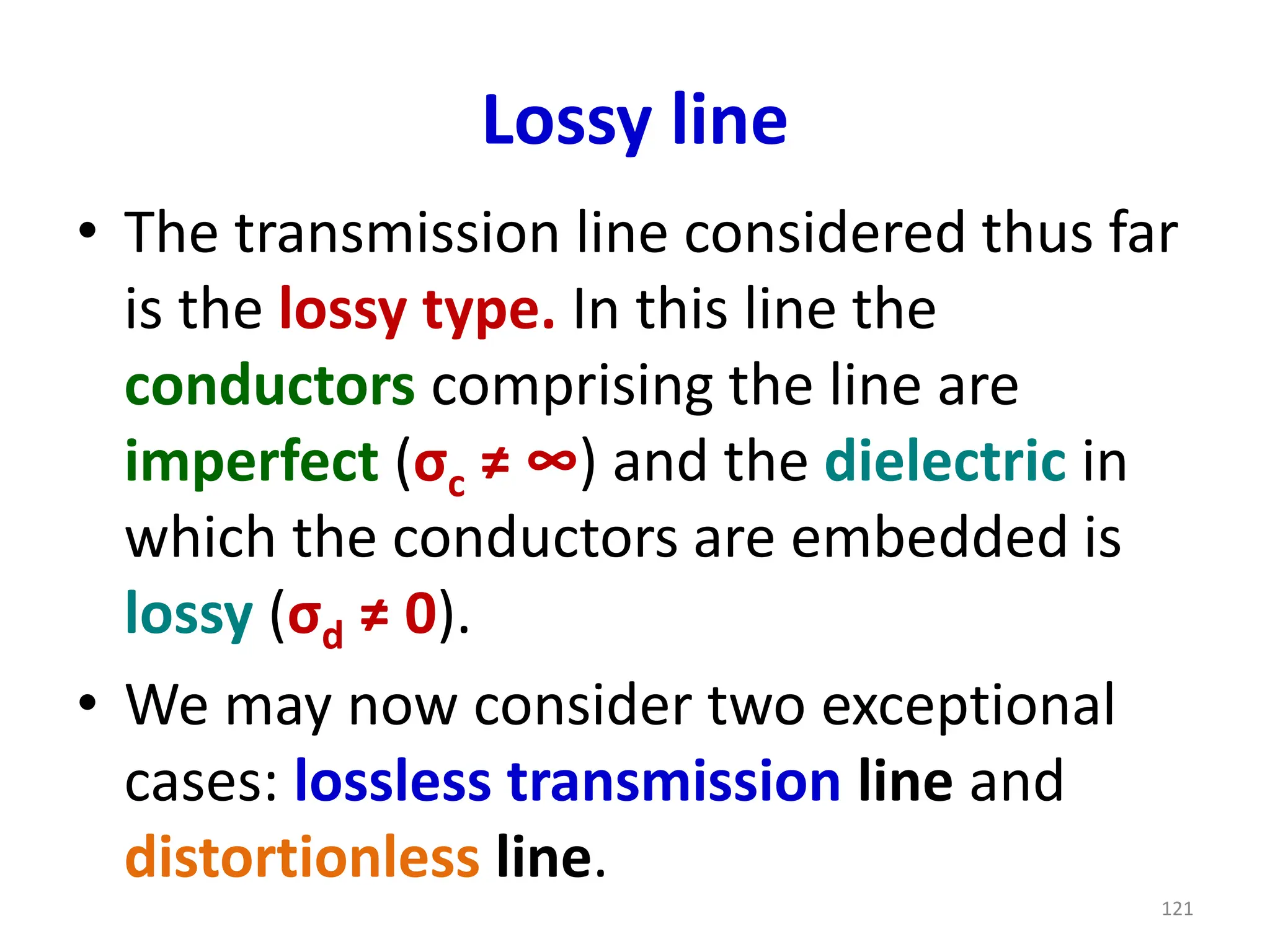
Lossy line
• Thetransmission line considered thus far
is the lossy type. In this line the
conductors comprising the line are
imperfect (σc ≠ ∞) and the dielectric in
which the conductors are embedded is
lossy (σd ≠ 0).
• We may now consider two exceptional
cases: lossless transmission line and
distortionless line.
121
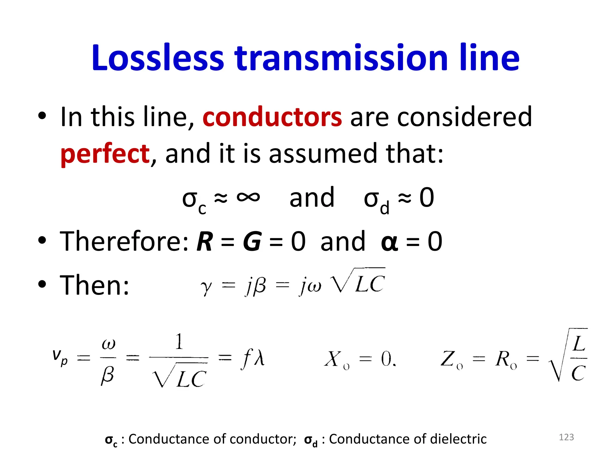
Lossless transmission line
•In this line, conductors are considered
perfect, and it is assumed that:
σc ≈ ∞ and σd ≈ 0
• Therefore: R = G = 0 and α = 0
• Then:
σc : Conductance of conductor; σd : Conductance of dielectric 123
vp
Distortionless line
• Asignal normally consists of a band of
frequencies and when passing through a
dissipative line the amplitude of the
different components will be attenuated
differently, because α depends on the
frequency. This results in distortion.
125
126.
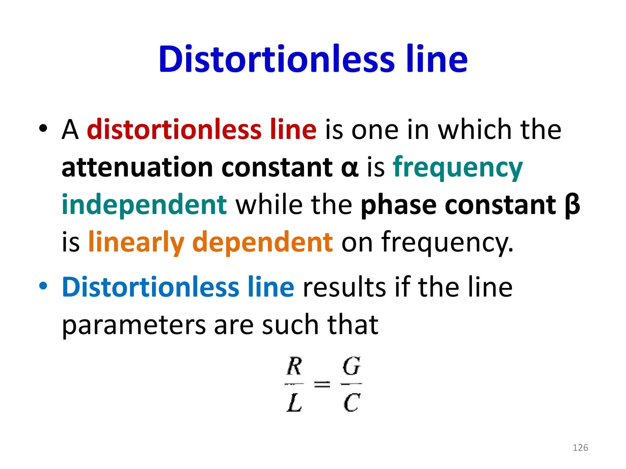
Distortionless line
• Adistortionless line is one in which the
attenuation constant α is frequency
independent while the phase constant β
is linearly dependent on frequency.
• Distortionless line results if the line
parameters are such that
126
127.
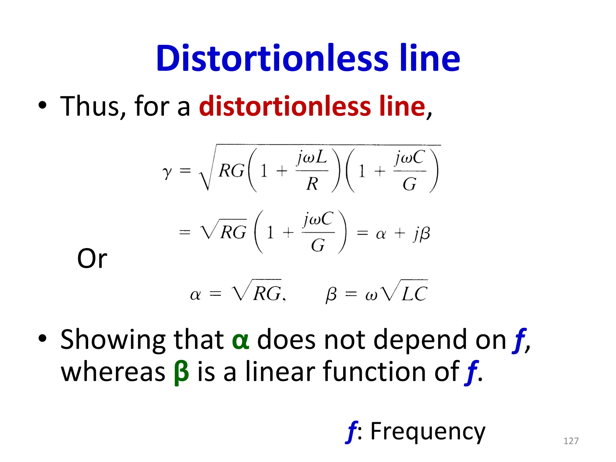
Distortionless line
• Thus,for a distortionless line,
• Showing that α does not depend on f,
whereas β is a linear function of f.
127
Or
f: Frequency
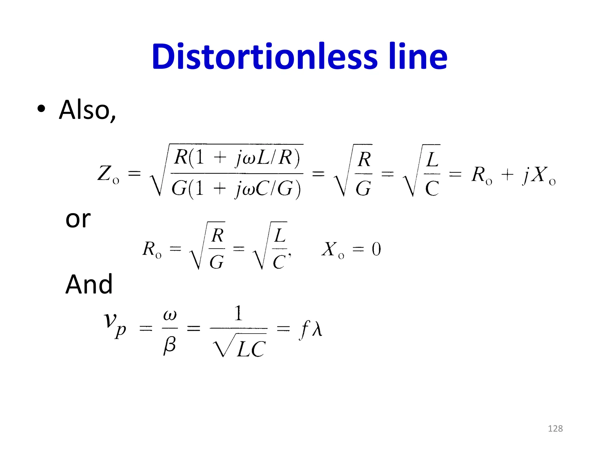
Distortionless line
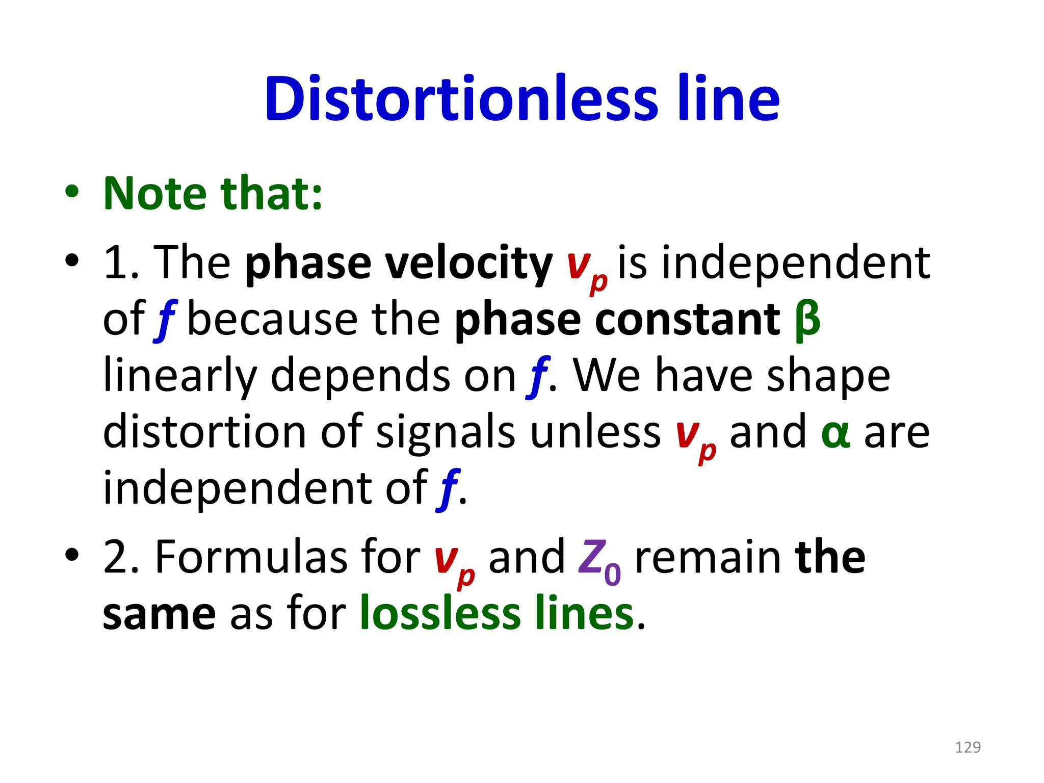
• Notethat:
• 1. The phase velocity vp is independent
of f because the phase constant β
linearly depends on f. We have shape
distortion of signals unless vp and α are
independent of f.
• 2. Formulas for vp and Z0 remain the
same as for lossless lines.
129
130.
Distortionless line
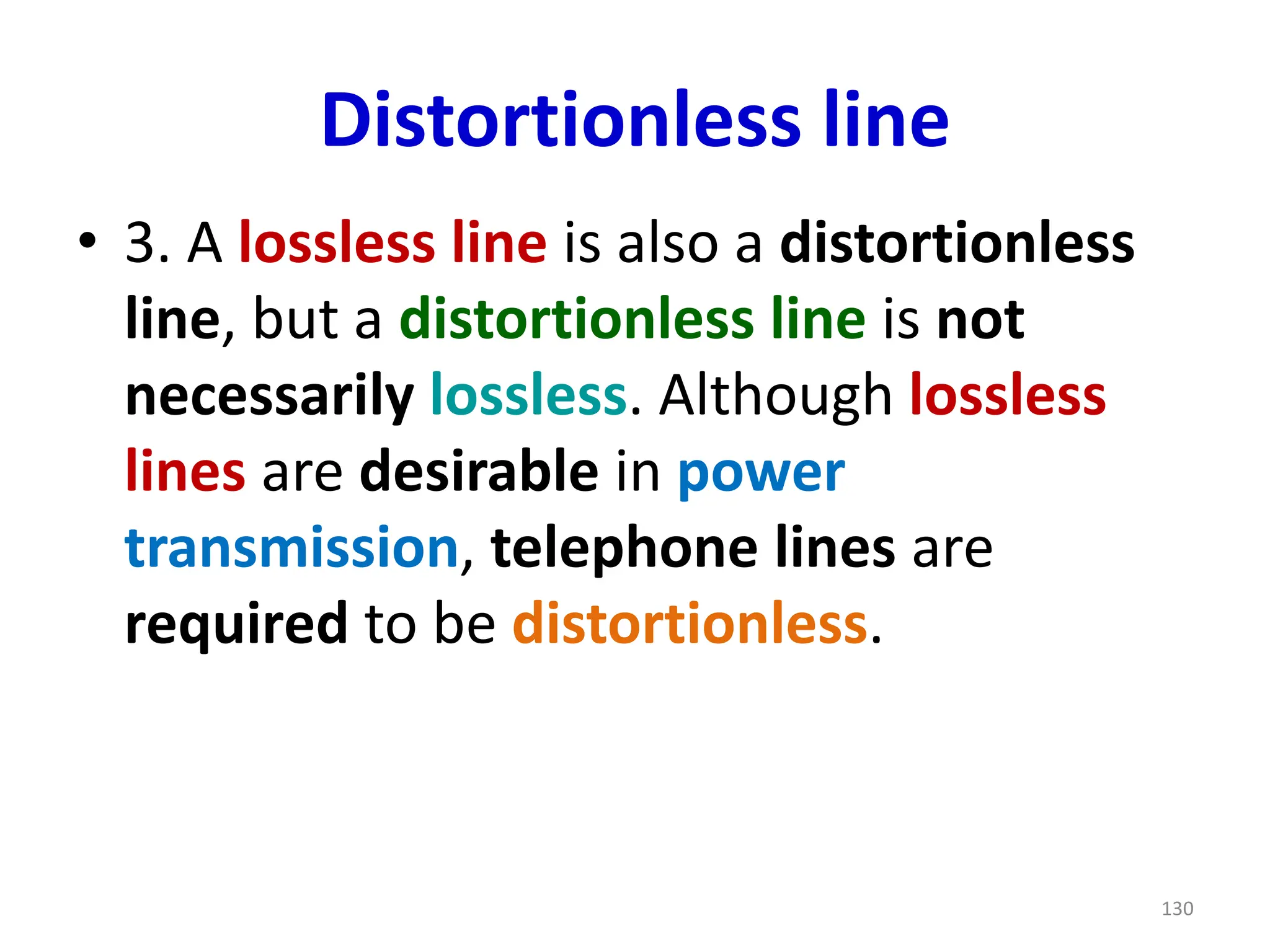
• 3.A lossless line is also a distortionless
line, but a distortionless line is not
necessarily lossless. Although lossless
lines are desirable in power
transmission, telephone lines are
required to be distortionless.
130
Propagation in matchedlines
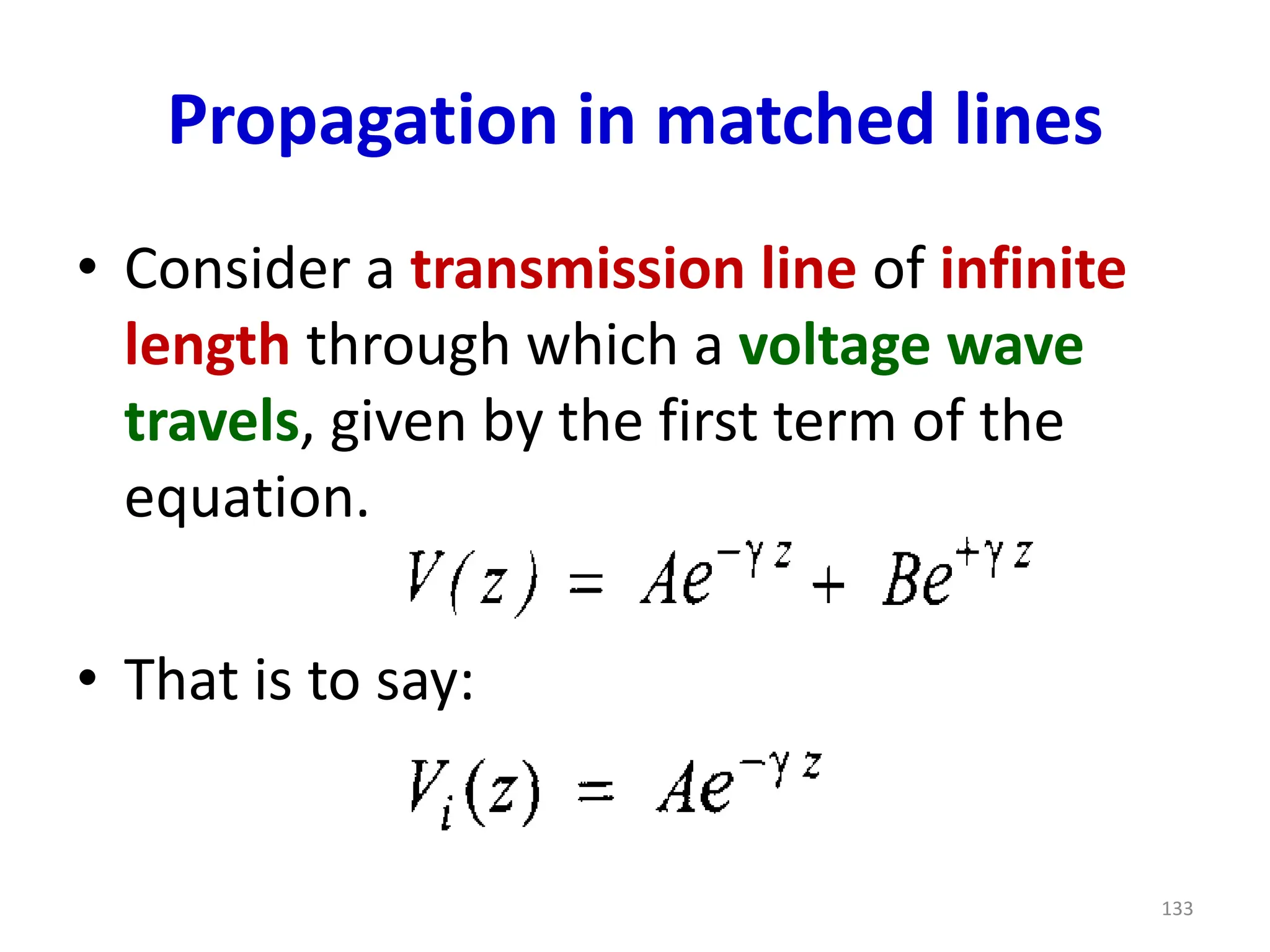
• Consider a transmission line of infinite
length through which a voltage wave
travels, given by the first term of the
equation.
• That is to say:
133
134.
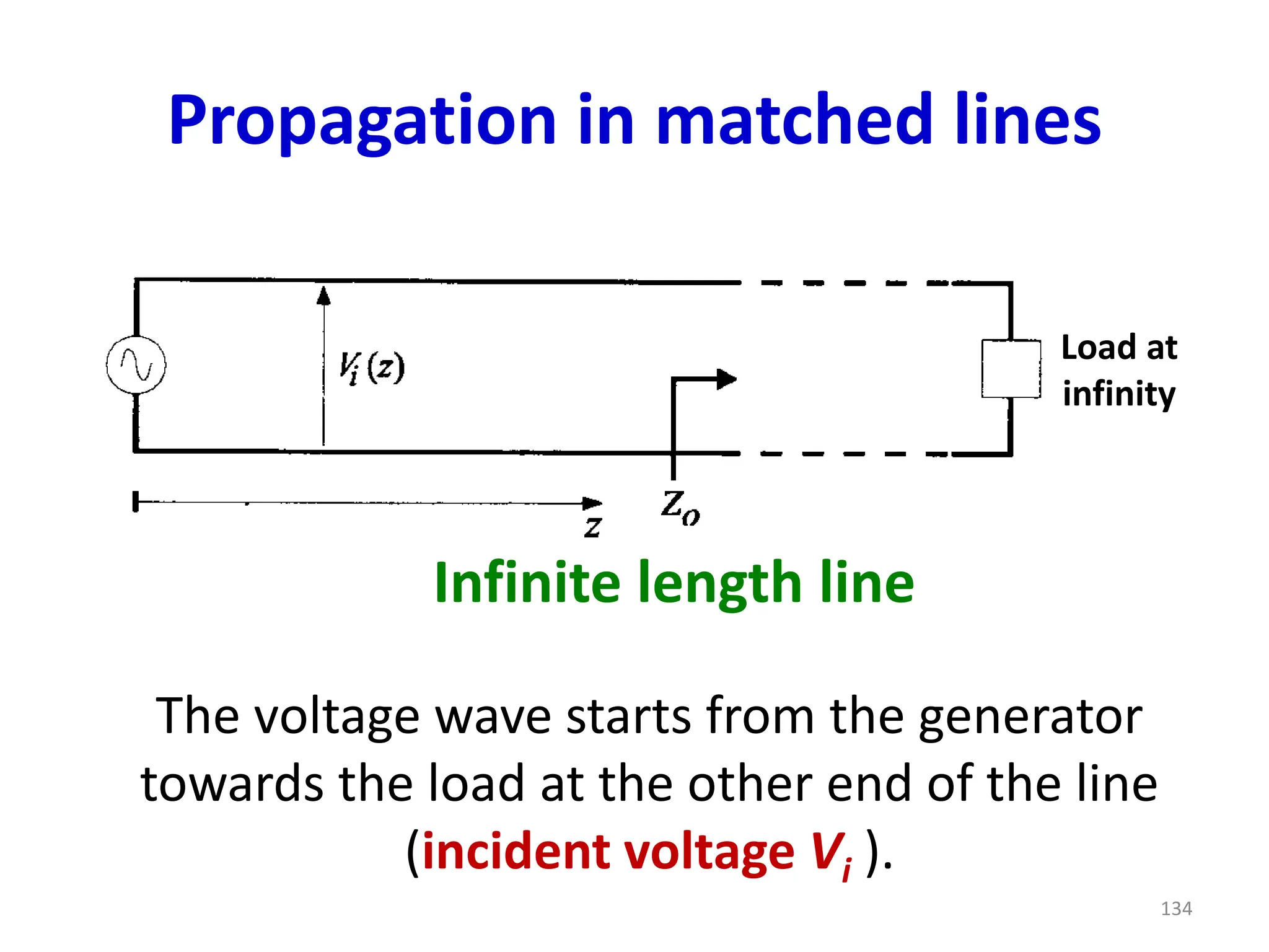
Propagation in matchedlines
The voltage wave starts from the generator
towards the load at the other end of the line
(incident voltage Vi ).
Infinite length line
134
Load at
infinity
135.
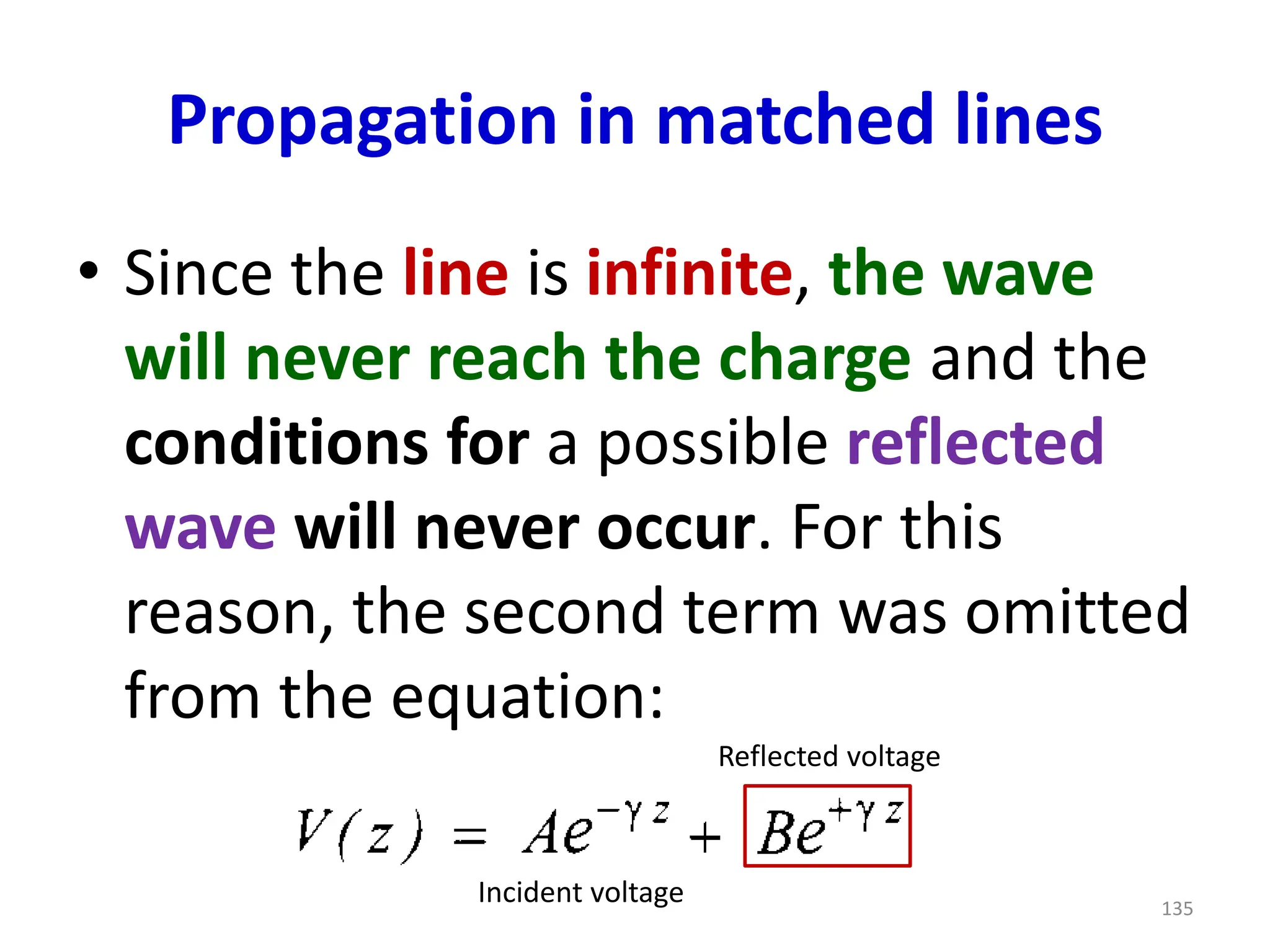
Propagation in matchedlines
• Since the line is infinite, the wave
will never reach the charge and the
conditions for a possible reflected
wave will never occur. For this
reason, the second term was omitted
from the equation:
135
Incident voltage
Reflected voltage
136.
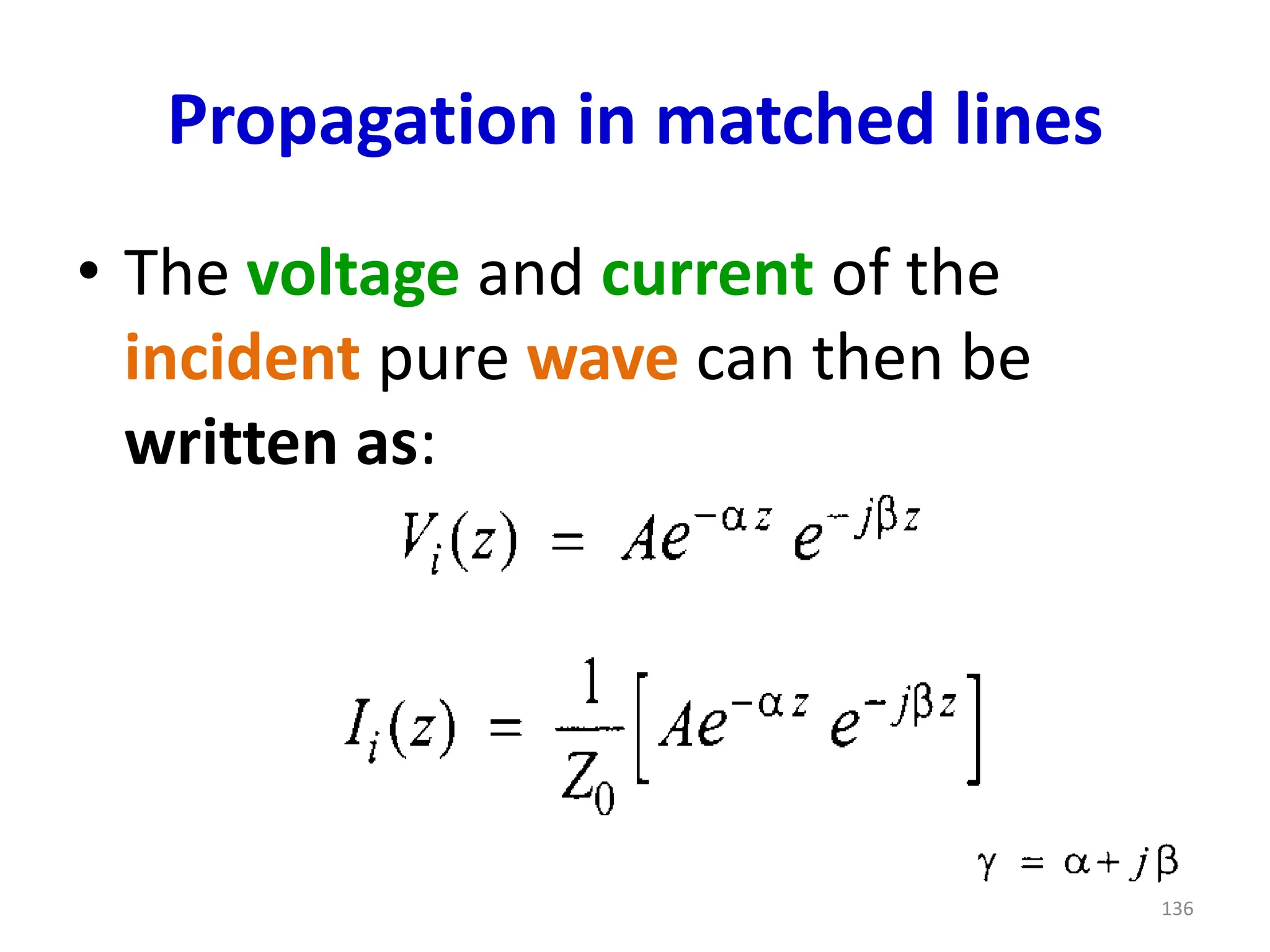
Propagation in matchedlines
• The voltage and current of the
incident pure wave can then be
written as:
136
137.
Propagation in matchedlines
• Regardless of the attenuation α of
the line, the ratio of voltage to
current is always equal to Z0.
• This result is independent of z, so it
is the same for all points on the line.
137
138.
Propagation in matchedlines
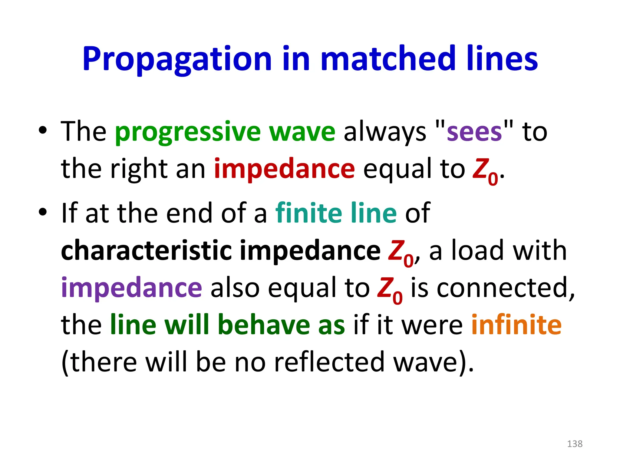
• The progressive wave always "sees" to
the right an impedance equal to Z0.
• If at the end of a finite line of
characteristic impedance Z0, a load with
impedance also equal to Z0 is connected,
the line will behave as if it were infinite
(there will be no reflected wave).
138
139.
Propagation in matchedlines
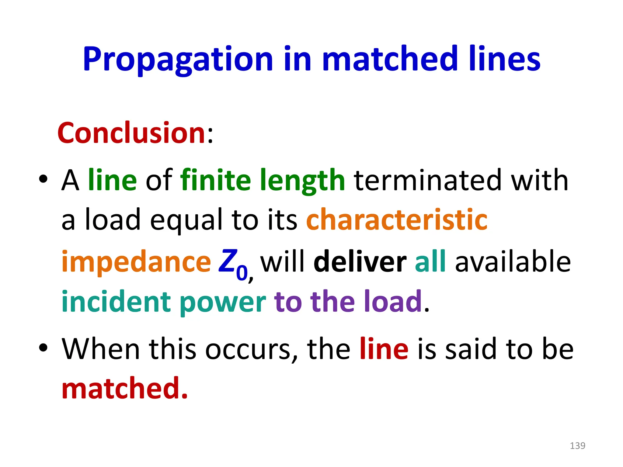
Conclusion:
• A line of finite length terminated with
a load equal to its characteristic
impedance Z0, will deliver all available
incident power to the load.
• When this occurs, the line is said to be
matched.
139
140.
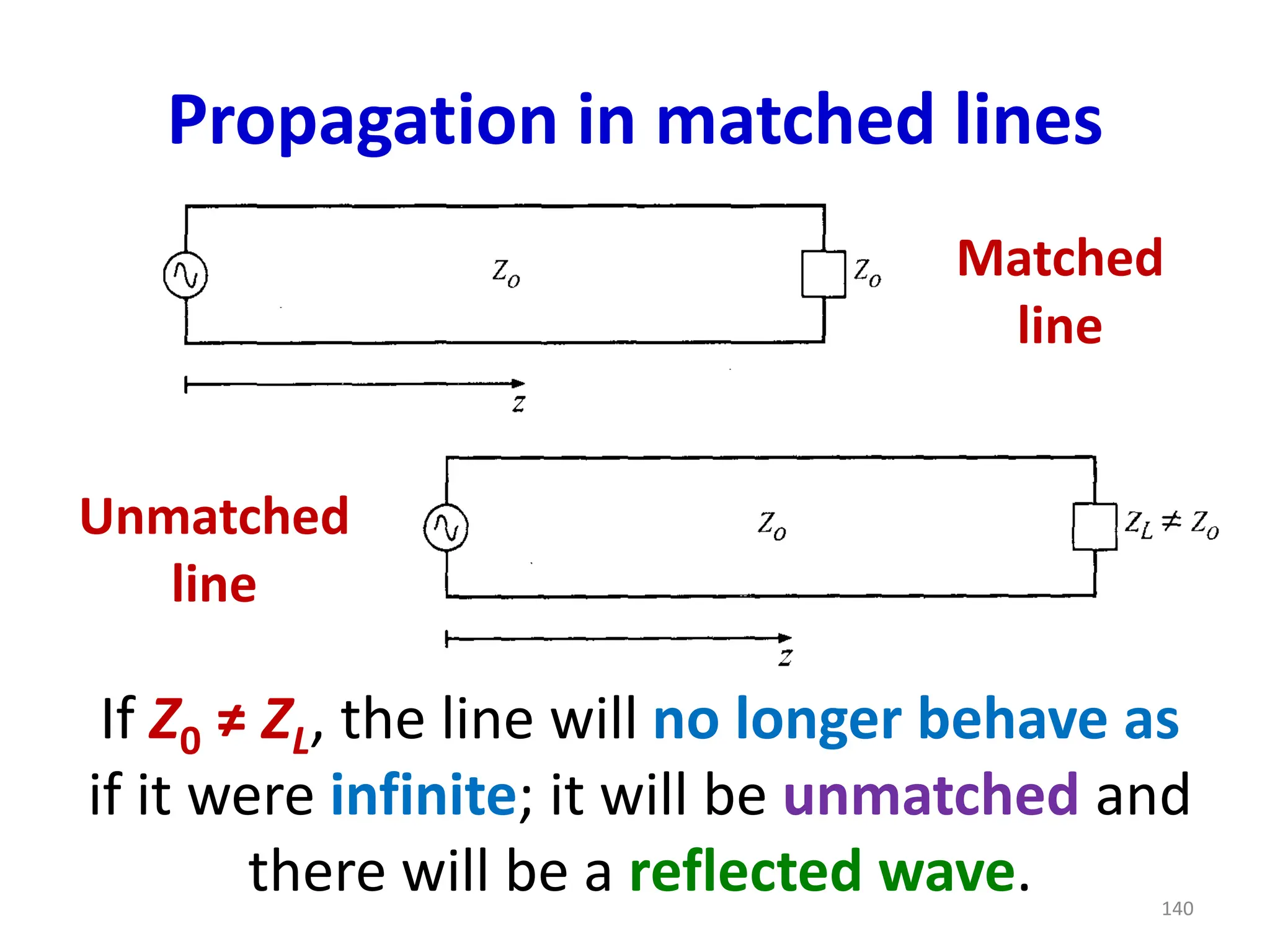
Propagation in matchedlines
Matched
line
If Z0 ≠ ZL, the line will no longer behave as
if it were infinite; it will be unmatched and
there will be a reflected wave.
Unmatched
line
140
141.
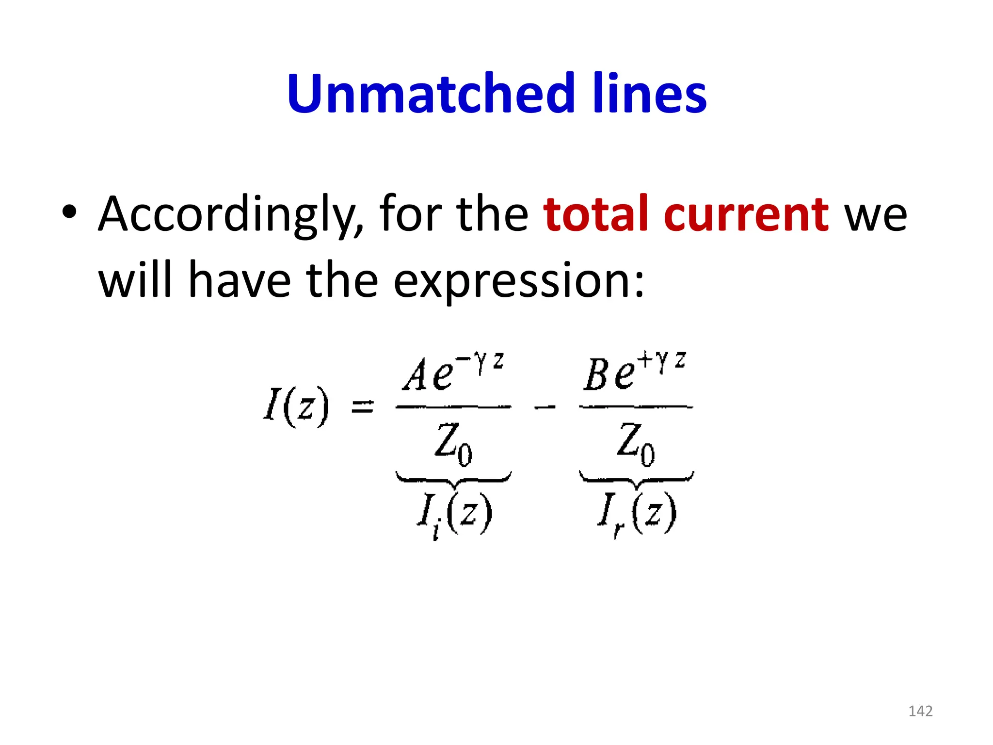
Unmatched lines
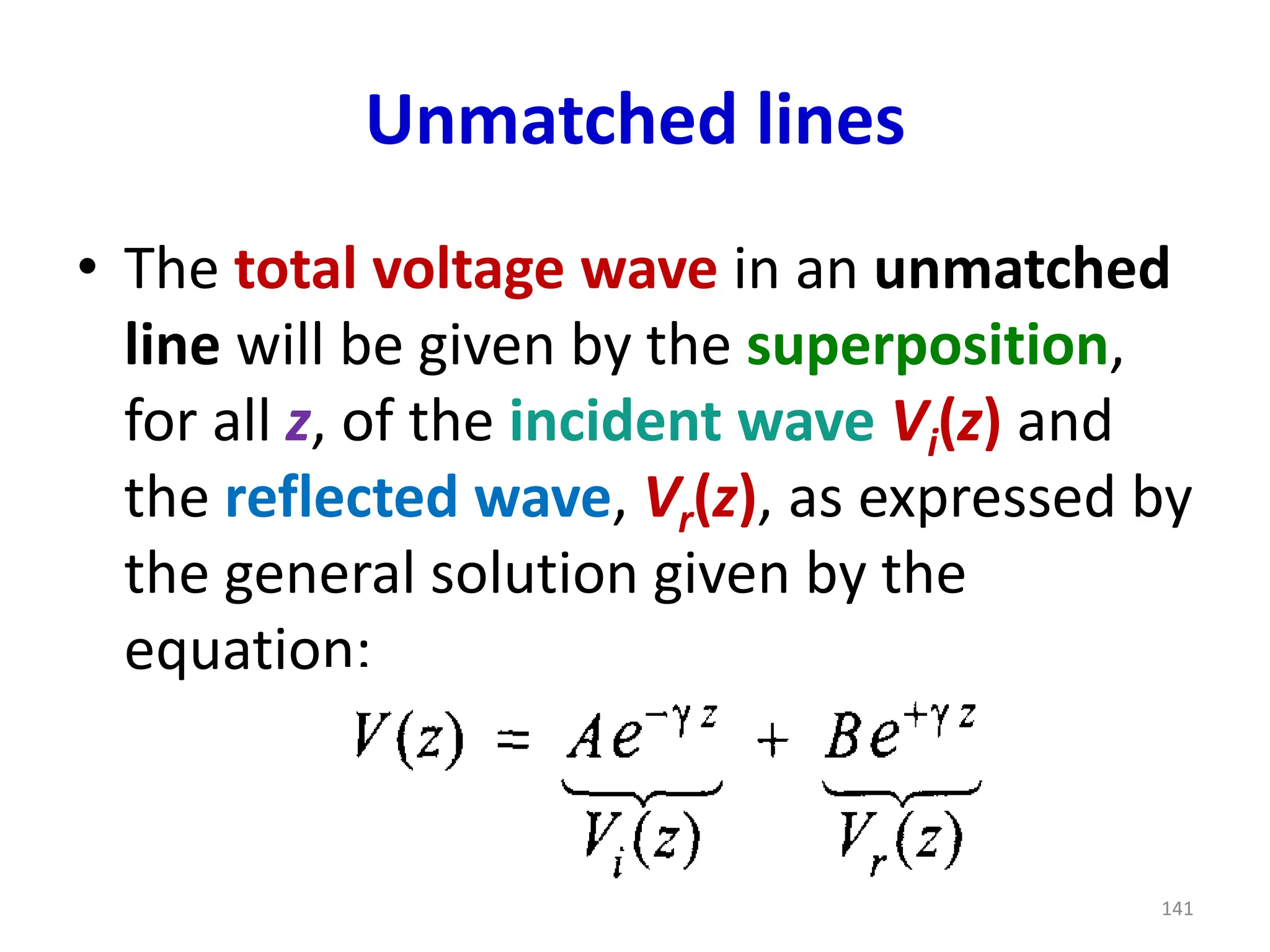
• Thetotal voltage wave in an unmatched
line will be given by the superposition,
for all z, of the incident wave Vi(z) and
the reflected wave, Vr(z), as expressed by
the general solution given by the
equation:
141
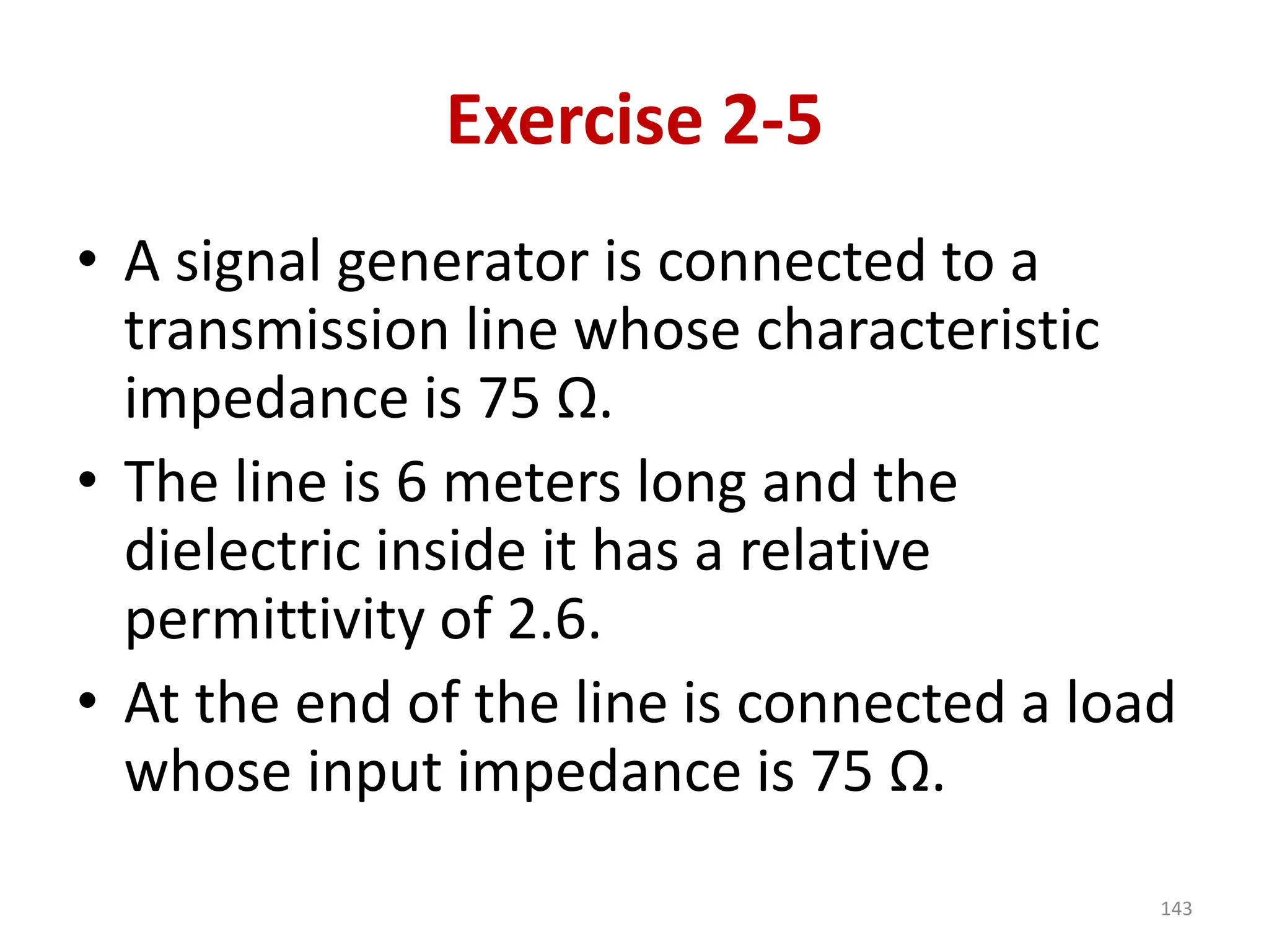
Exercise 2-5
• Asignal generator is connected to a
transmission line whose characteristic
impedance is 75 Ω.
• The line is 6 meters long and the
dielectric inside it has a relative
permittivity of 2.6.
• At the end of the line is connected a load
whose input impedance is 75 Ω.
143
144.
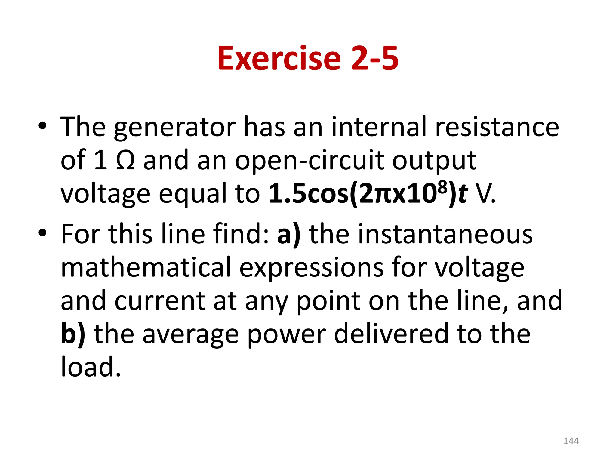
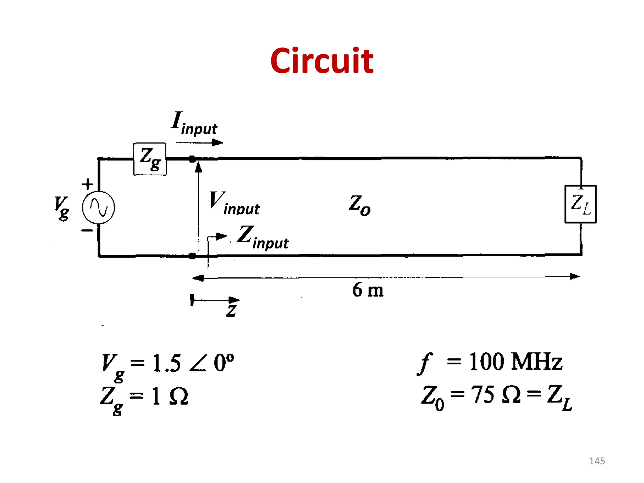
Exercise 2-5
• Thegenerator has an internal resistance
of 1 Ω and an open-circuit output
voltage equal to 1.5cos(2πx108)t V.
• For this line find: a) the instantaneous
mathematical expressions for voltage
and current at any point on the line, and
b) the average power delivered to the
load.
144
Solution
• Since theline is matched, the impedance
seen at all points on the line is the same,
and therefore the input impedance is 75
ohms:
Zinput = 75 Ω
146
147.
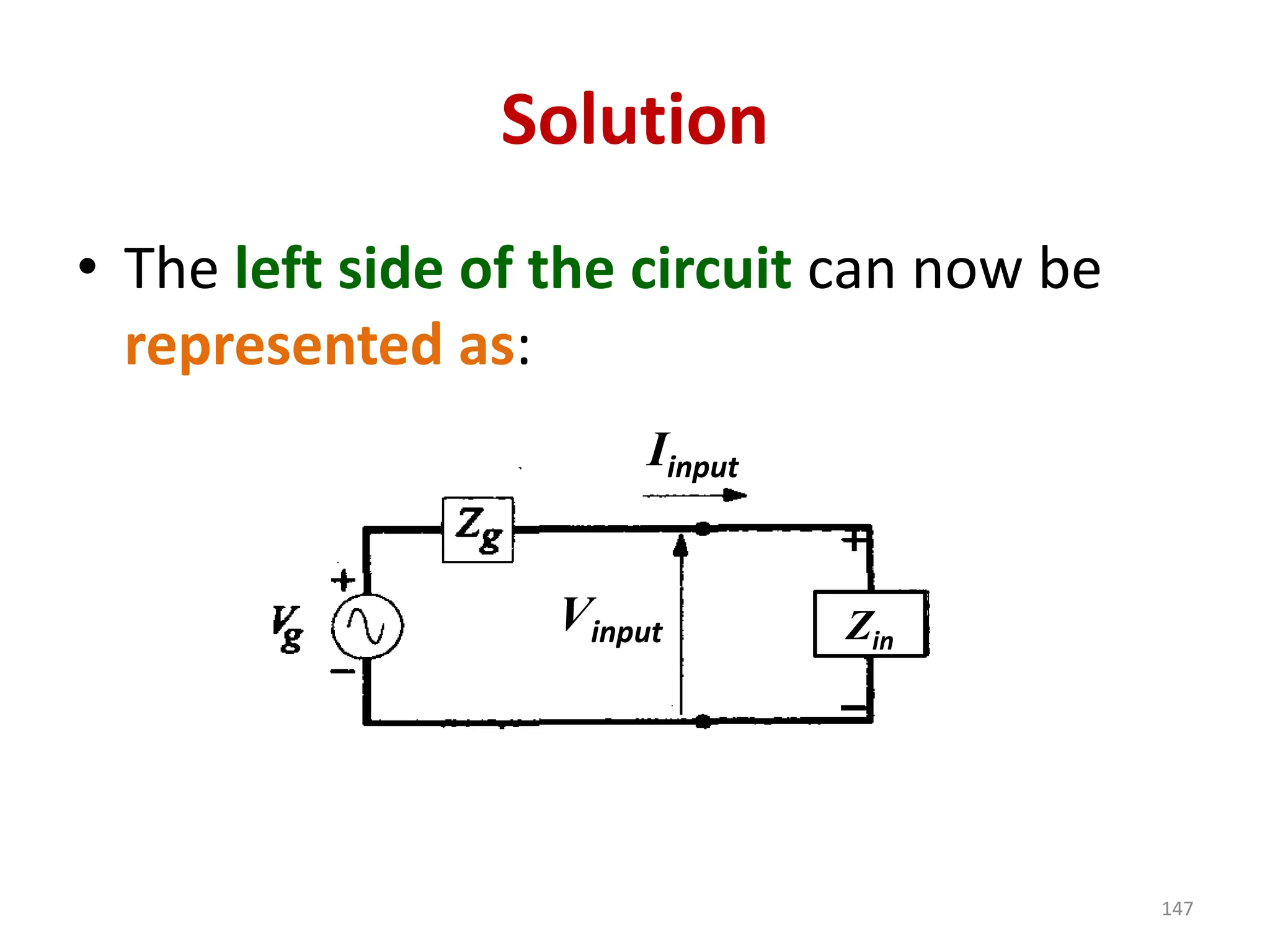
Solution
• The leftside of the circuit can now be
represented as:
147
Iinput
Vinput Zin
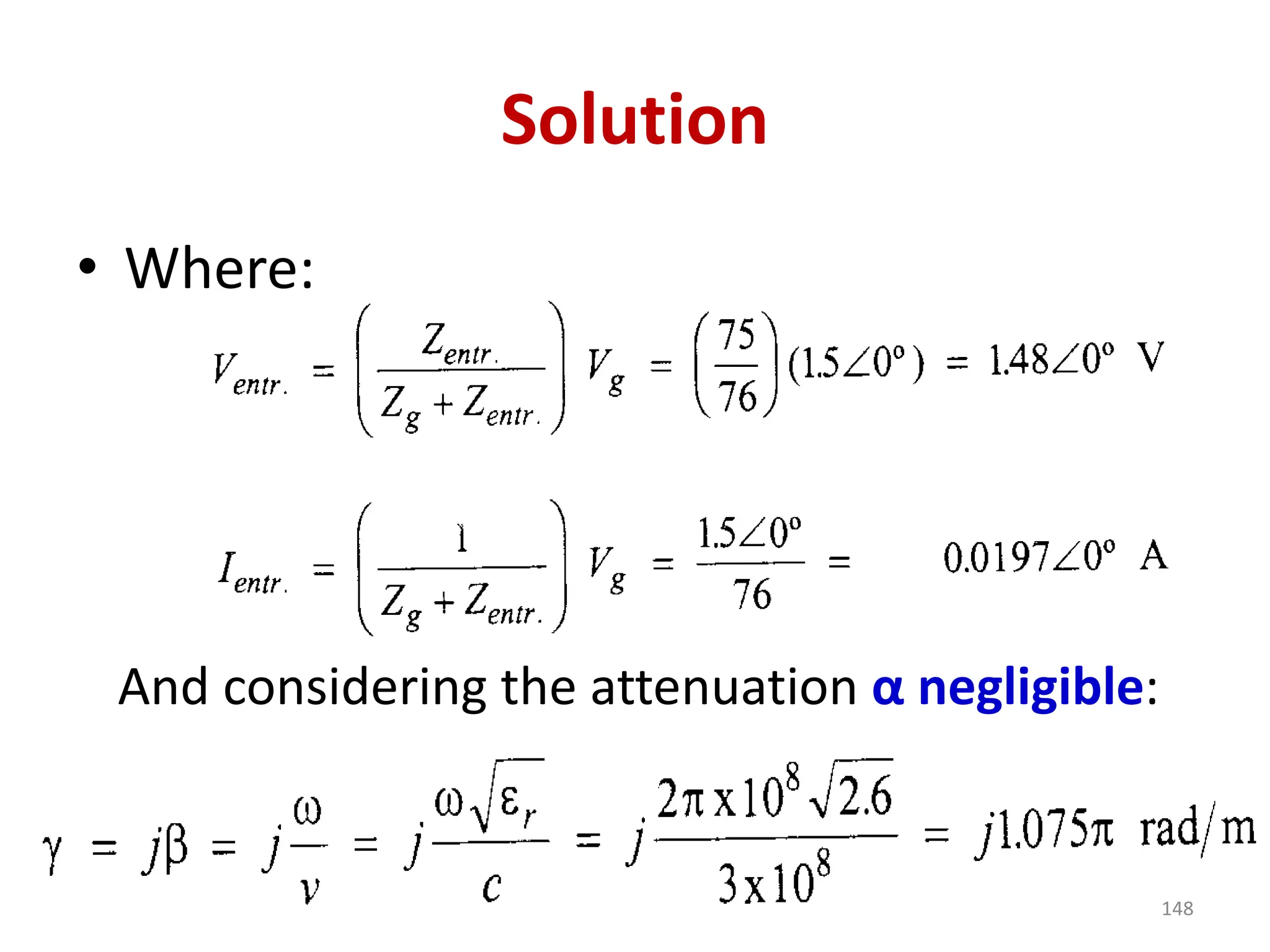
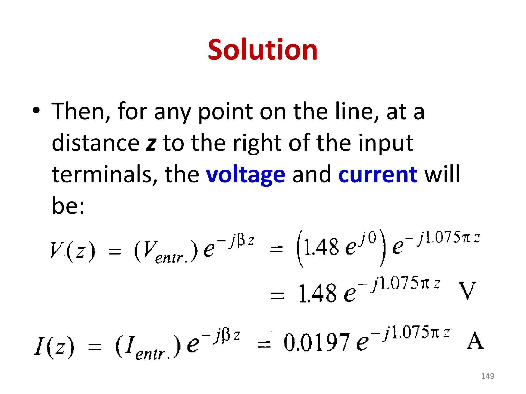
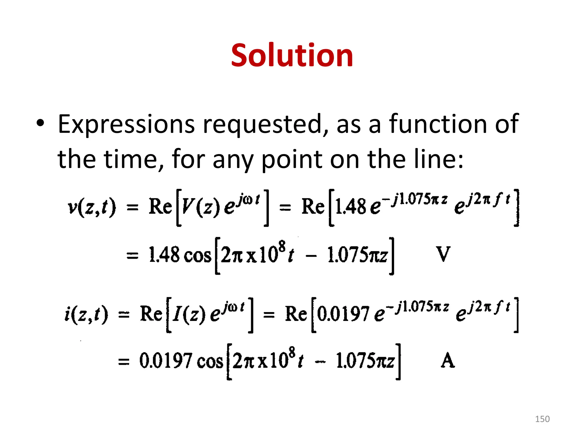
Solution
• Thus, forexample, for the specific point
where the load is, instantaneous
expressions are obtained by substituting
z = 6 m into the above equations.
• As regards the average power delivered
to the load, this must be equal to the
average input power, [considering
lossless line (α = 0)].
151
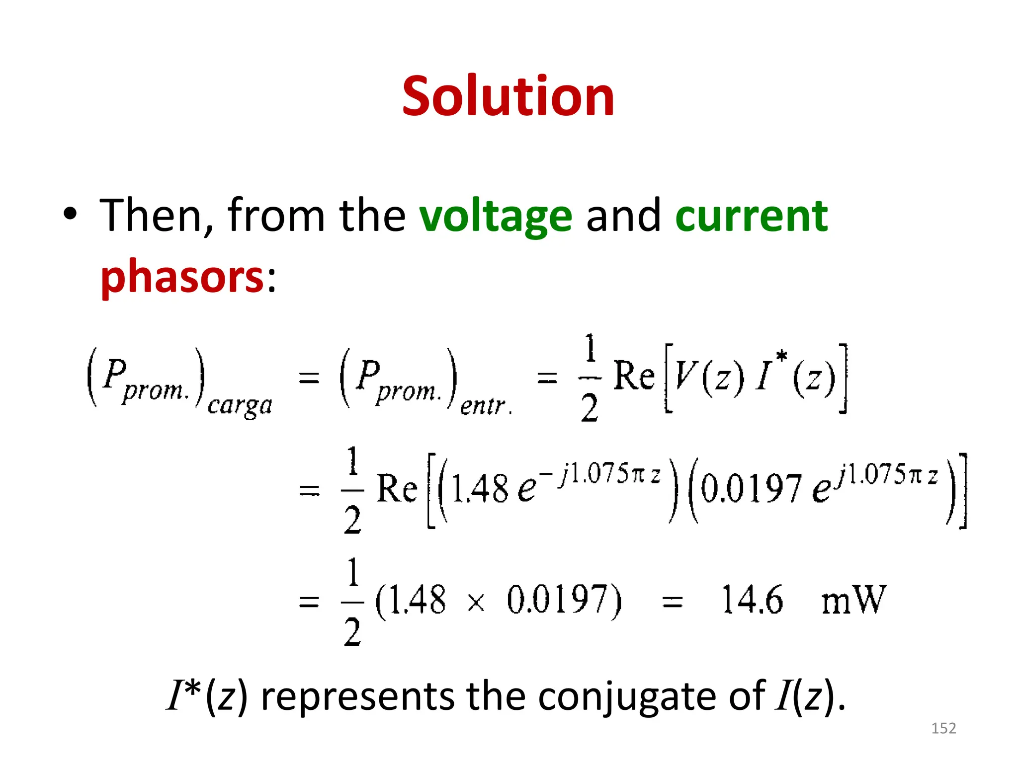
152.
Solution
• Then, fromthe voltage and current
phasors:
I*(z) represents the conjugate of I(z).
152
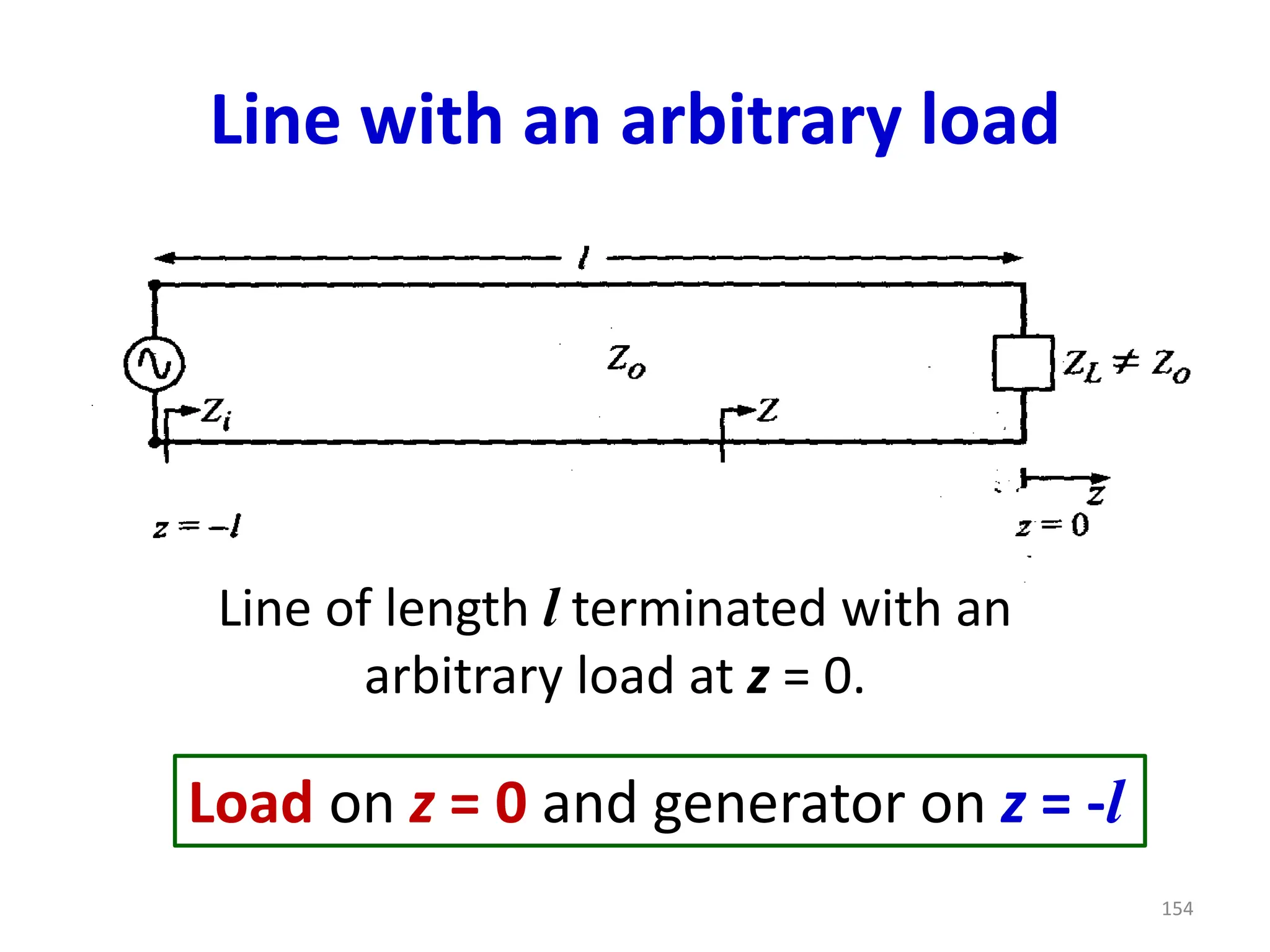
Line with anarbitrary load
Line of length l terminated with an
arbitrary load at z = 0.
Load on z = 0 and generator on z = -l
154
155.
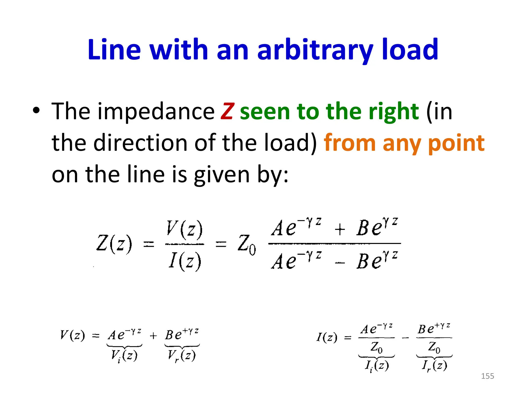
Line with anarbitrary load
• The impedance Z seen to the right (in
the direction of the load) from any point
on the line is given by:
155
156.
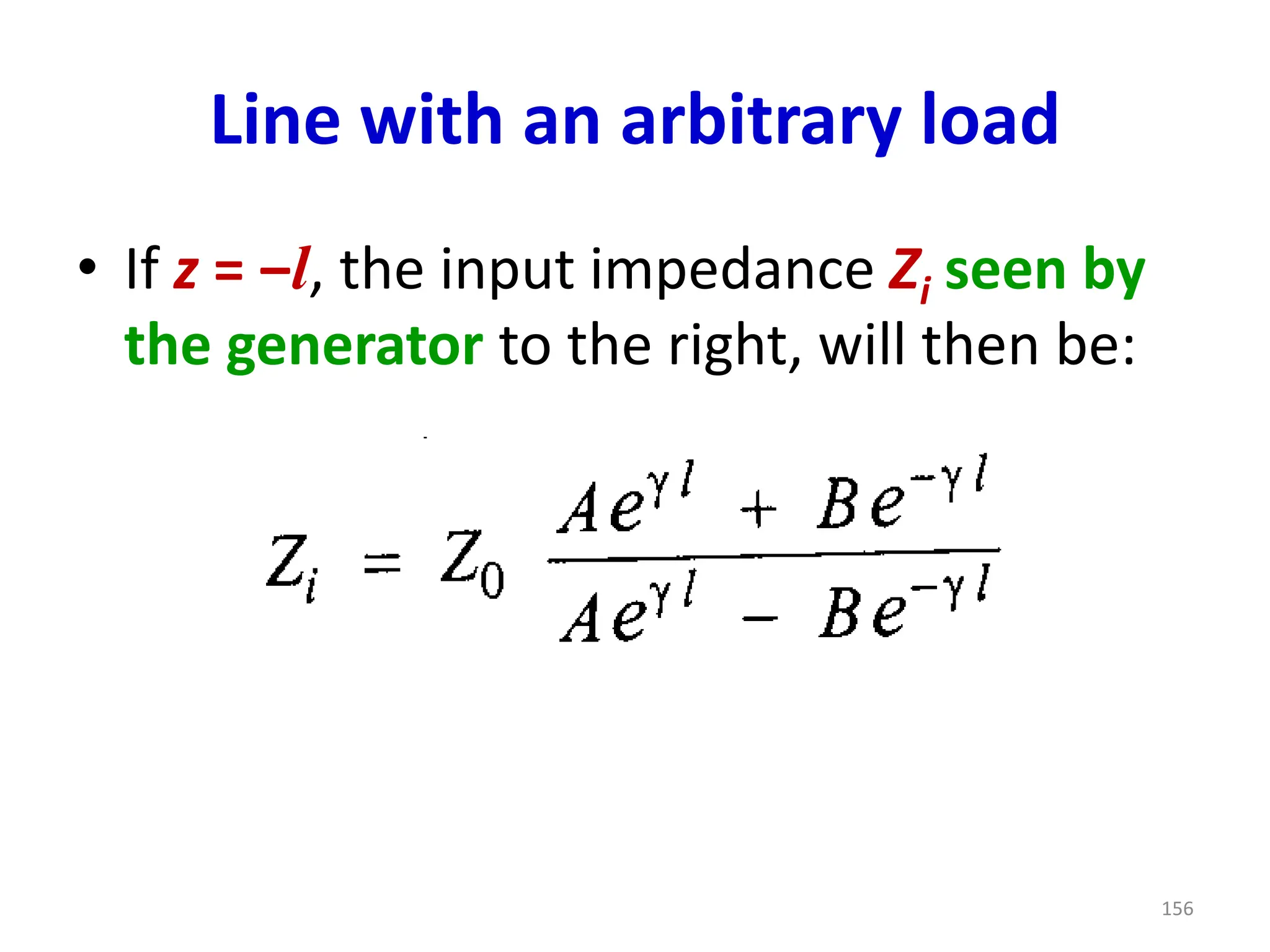
Line with anarbitrary load
• If z = ‒l, the input impedance Zi seen by
the generator to the right, will then be:
156
157.
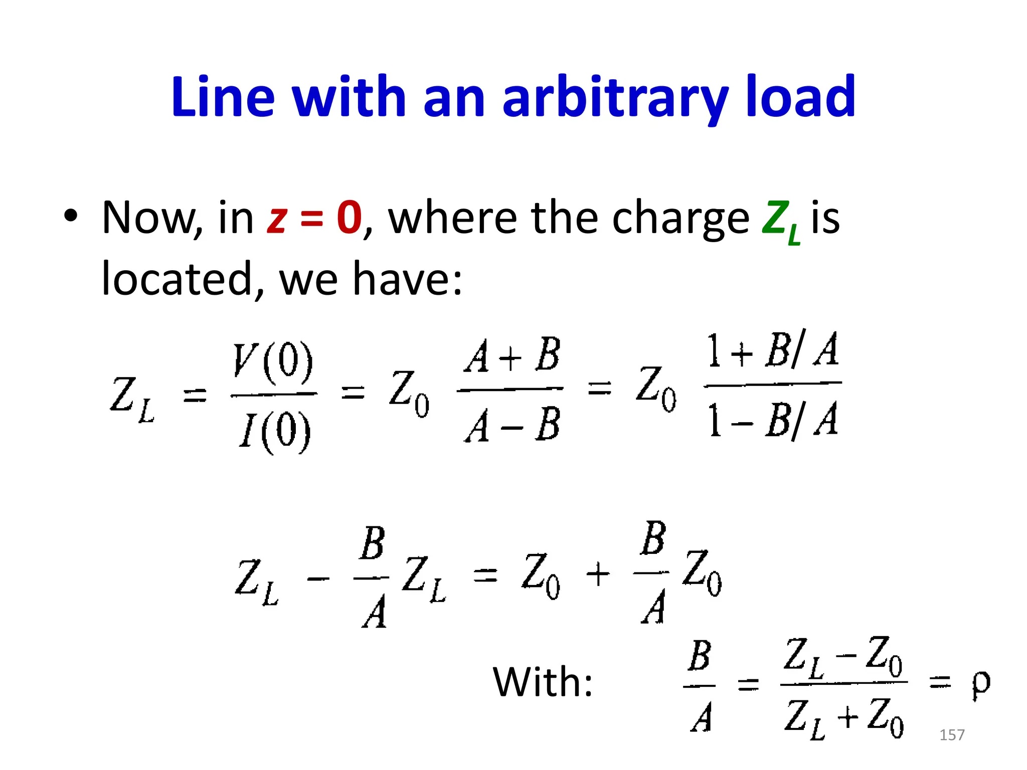
Line with anarbitrary load
• Now, in z = 0, where the charge ZL is
located, we have:
With:
157
158.
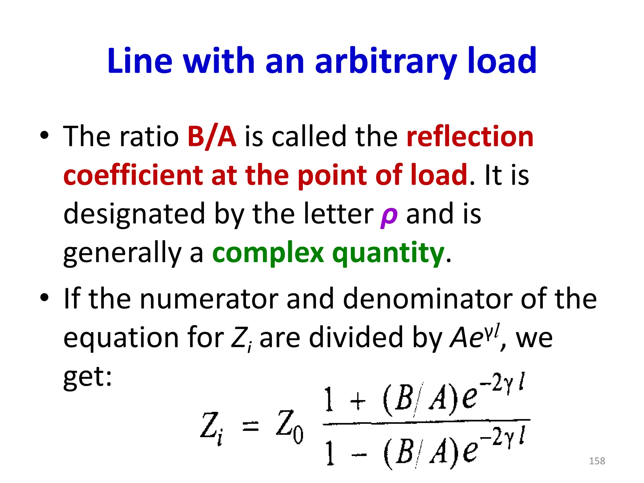
Line with anarbitrary load
• The ratio B/A is called the reflection
coefficient at the point of load. It is
designated by the letter ρ and is
generally a complex quantity.
• If the numerator and denominator of the
equation for Zi are divided by Aeγl, we
get:
158
159.
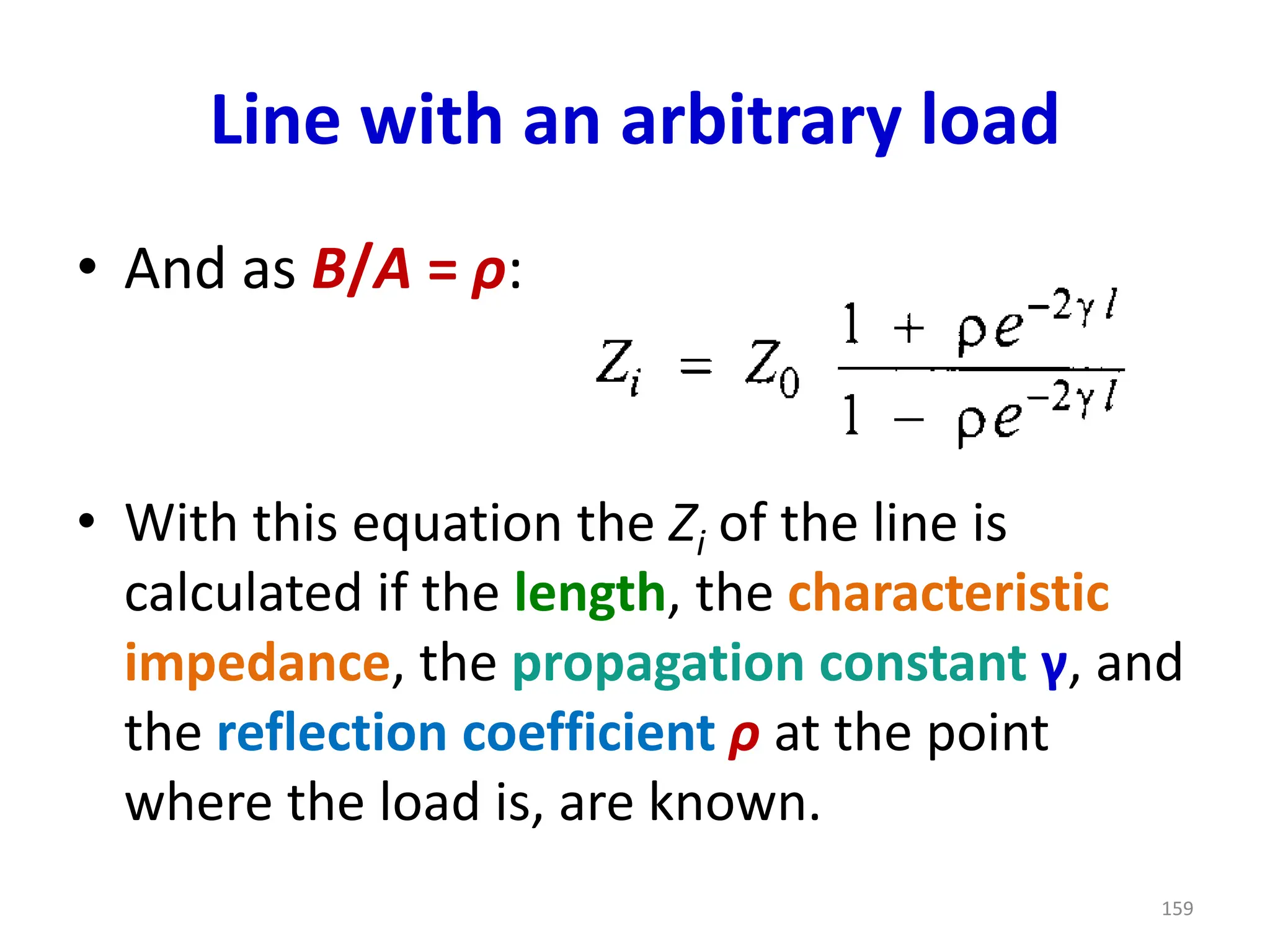
Line with anarbitrary load
• And as B/A = ρ:
• With this equation the Zi of the line is
calculated if the length, the characteristic
impedance, the propagation constant γ, and
the reflection coefficient ρ at the point
where the load is, are known.
159
160.
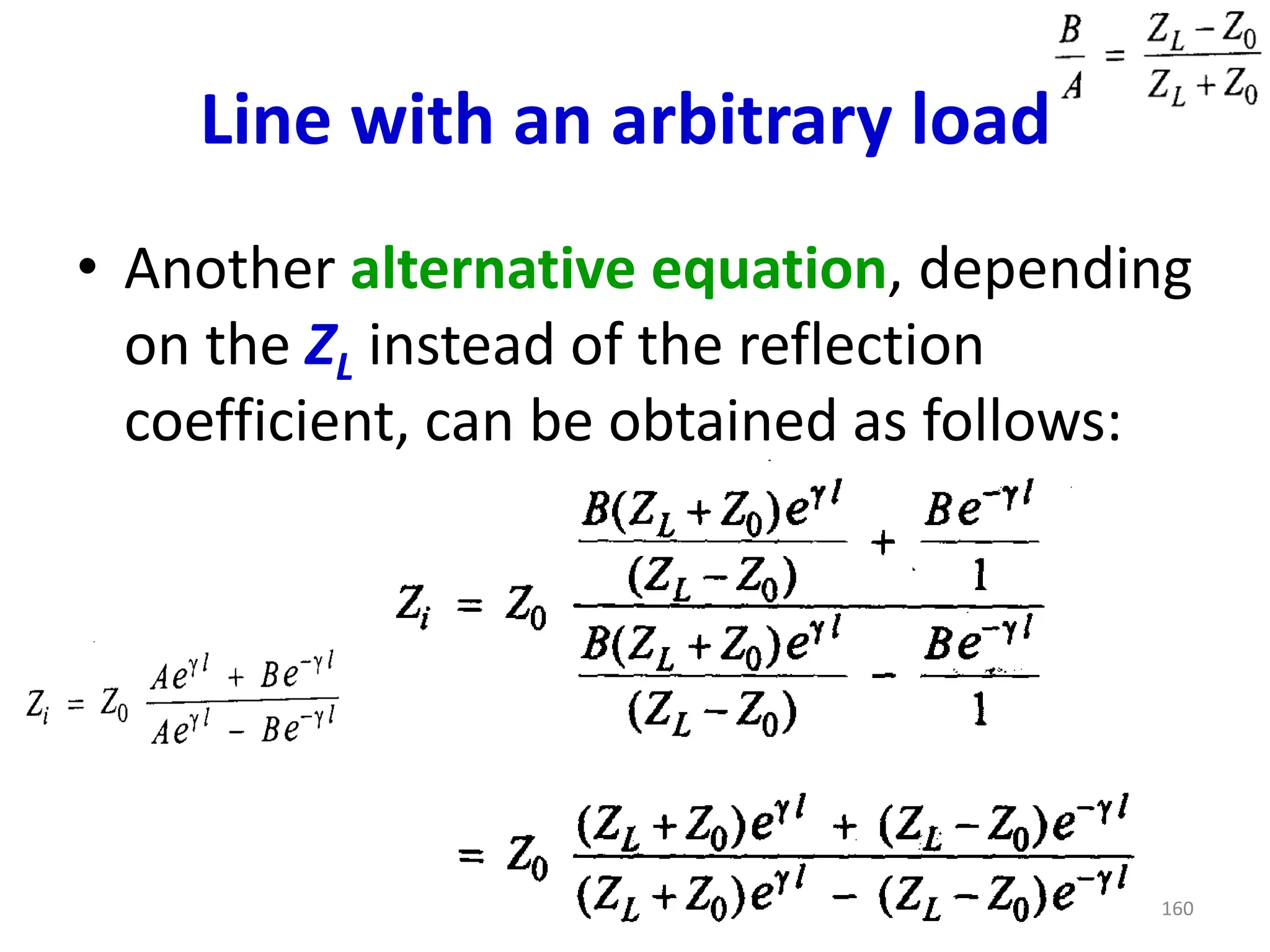
Line with anarbitrary load
• Another alternative equation, depending
on the ZL instead of the reflection
coefficient, can be obtained as follows:
160
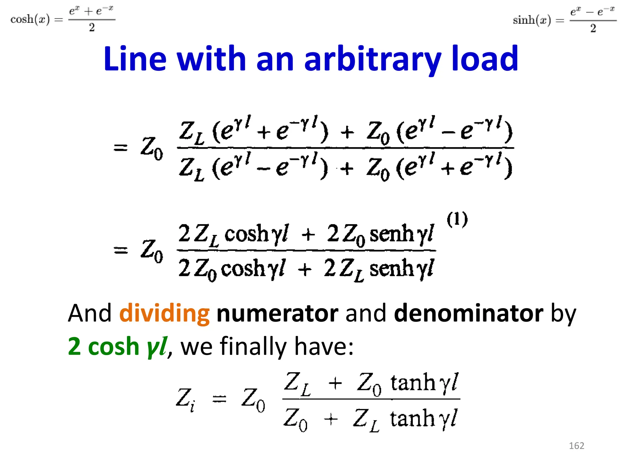
Line with anarbitrary load
And dividing numerator and denominator by
2 cosh γl, we finally have:
162
163.
Exercise 2-6
• Considera lossless transmission line,
with paper as a dielectric (εr = 3), which
works at a frequency of 300 MHz.
• The length of the line is 10 m and its
characteristic impedance is equal to 50
Ω.
• At the end of the line is connected a load
whose impedance is 80 Ω.
163
164.
Exercise 2-6
• Findthe voltages reflection
coefficient in the load and the input
impedance of the line.
• Also calculate the impedance that
would be seen at distances of λ/2
and λ, measured from the generator
to the load.
164
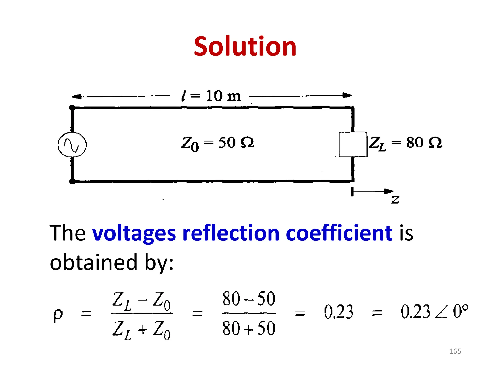
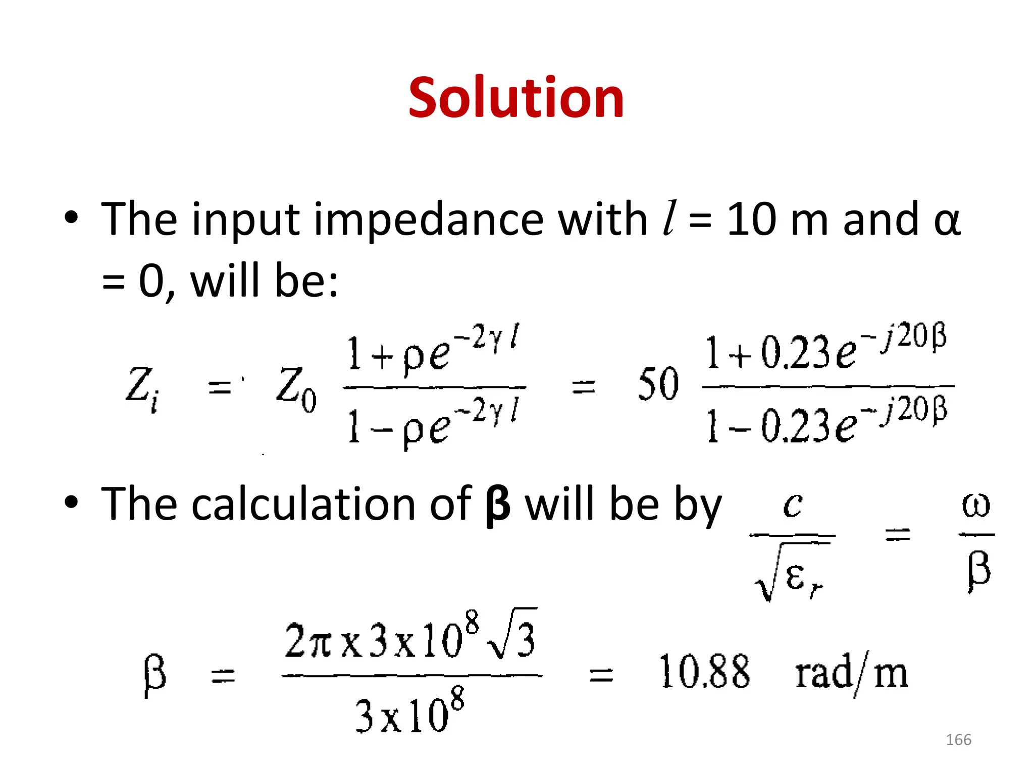
Solution
• The inputimpedance with l = 10 m and α
= 0, will be:
• The calculation of β will be by :
166
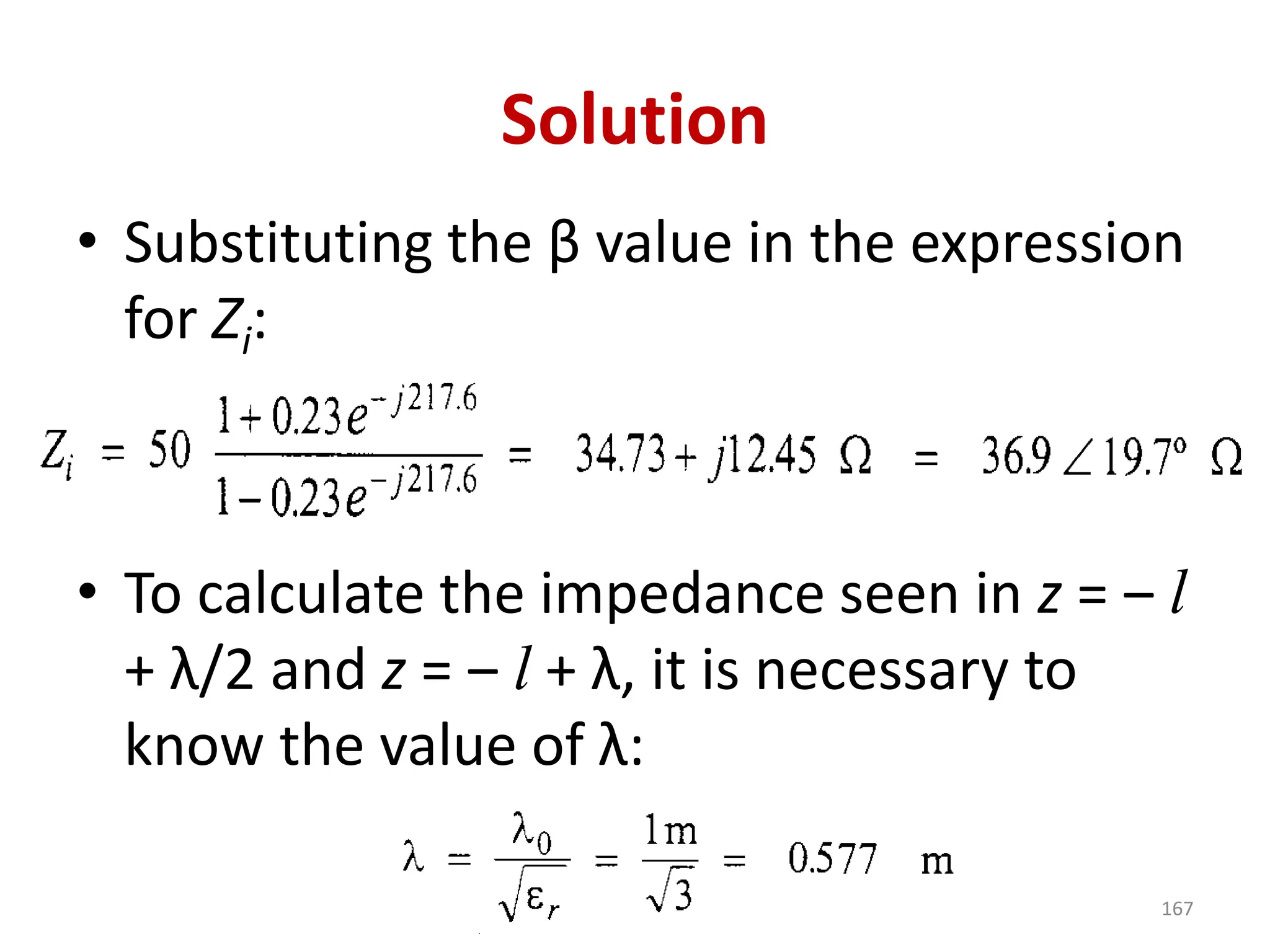
167.
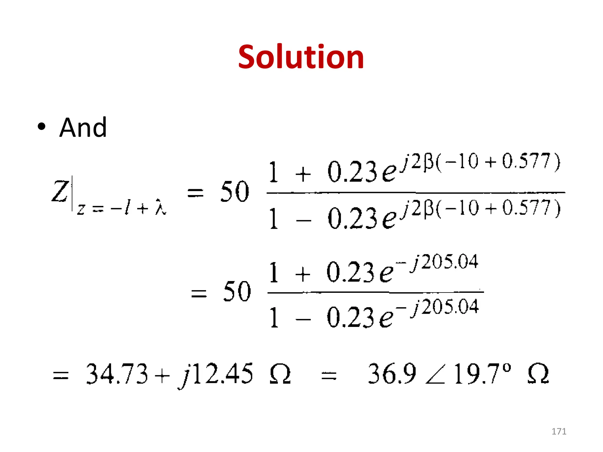
Solution
• Substituting theβ value in the expression
for Zi:
• To calculate the impedance seen in z = ‒ l
+ λ/2 and z = ‒ l + λ, it is necessary to
know the value of λ:
167
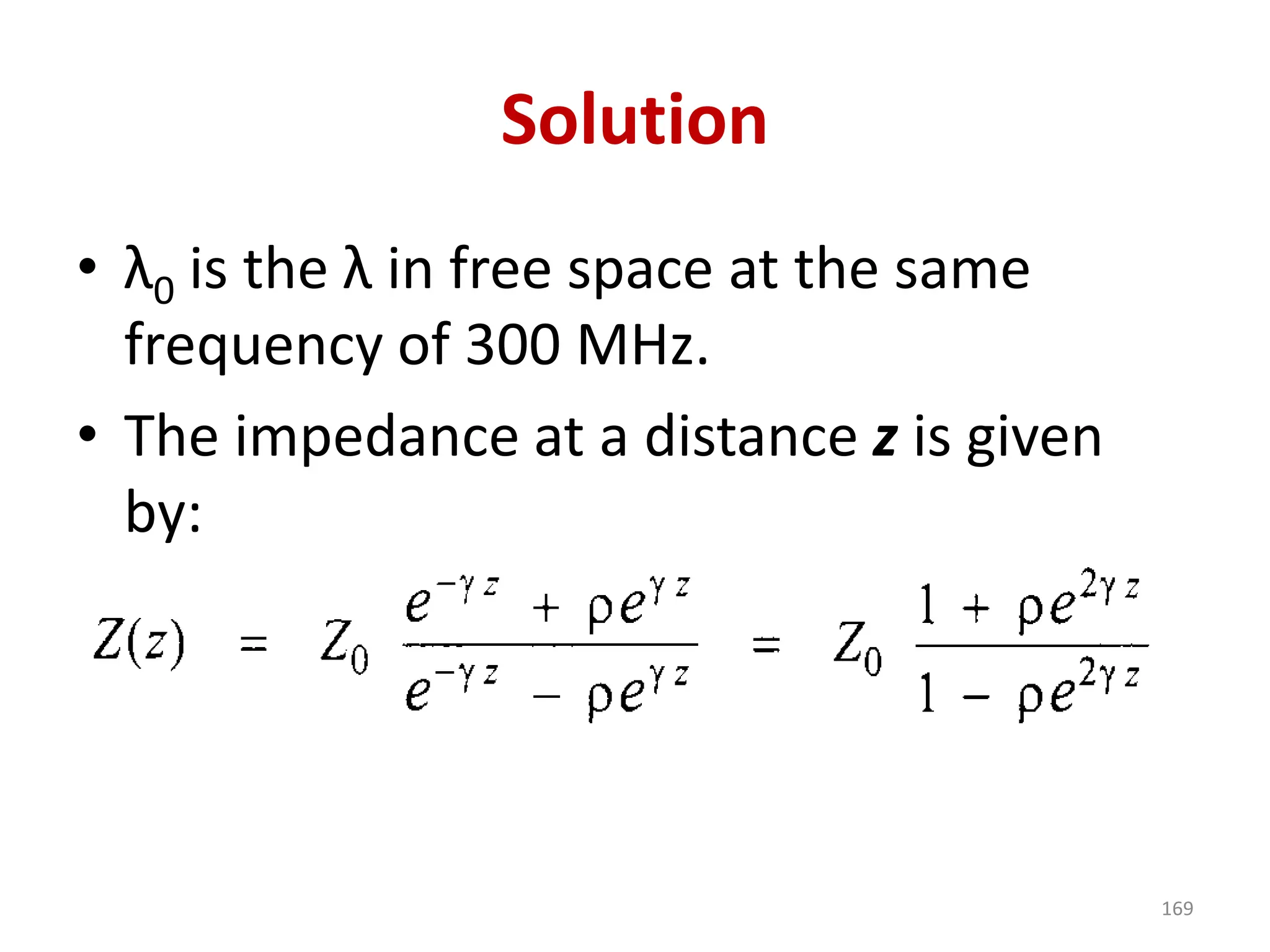
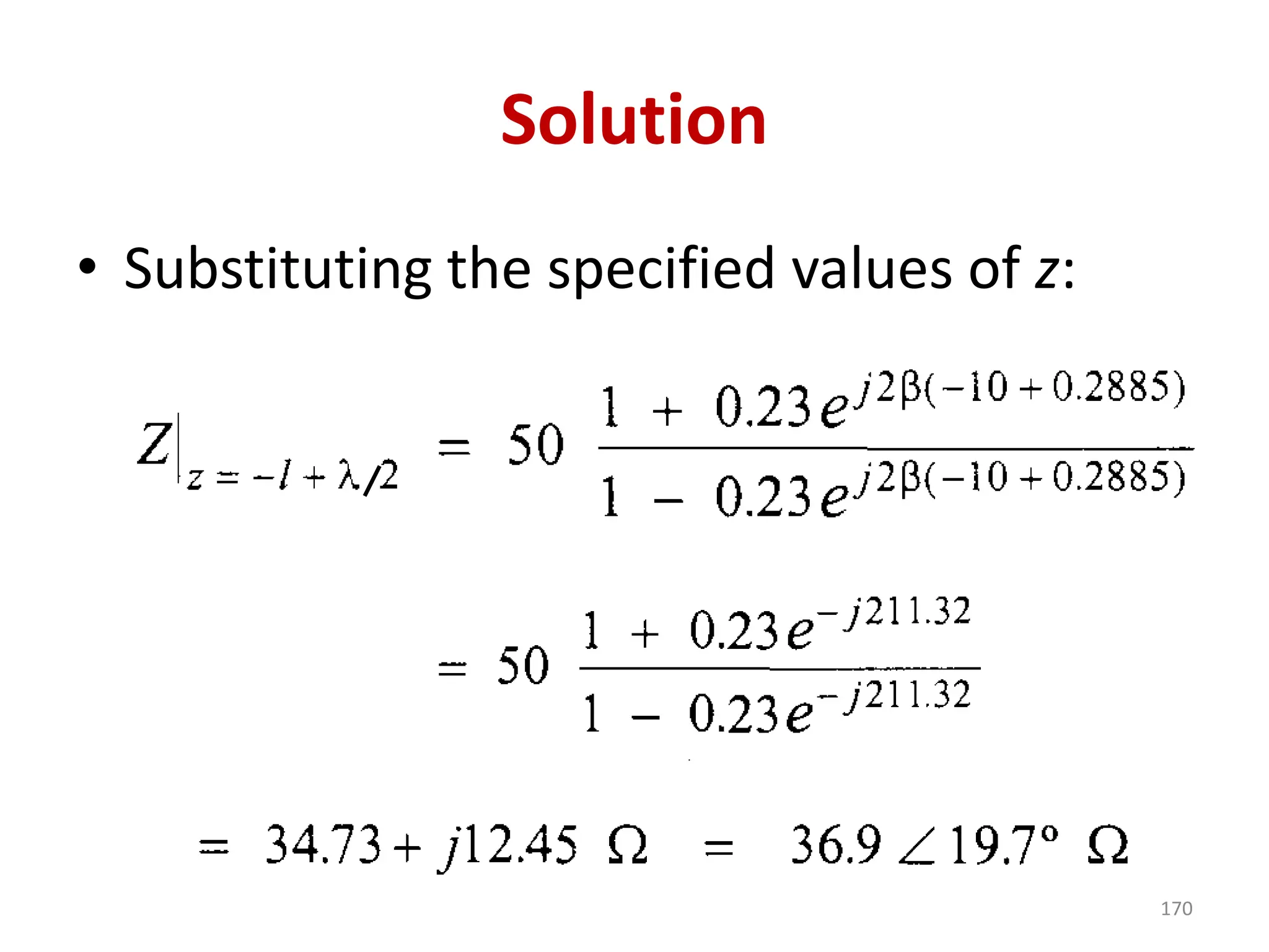
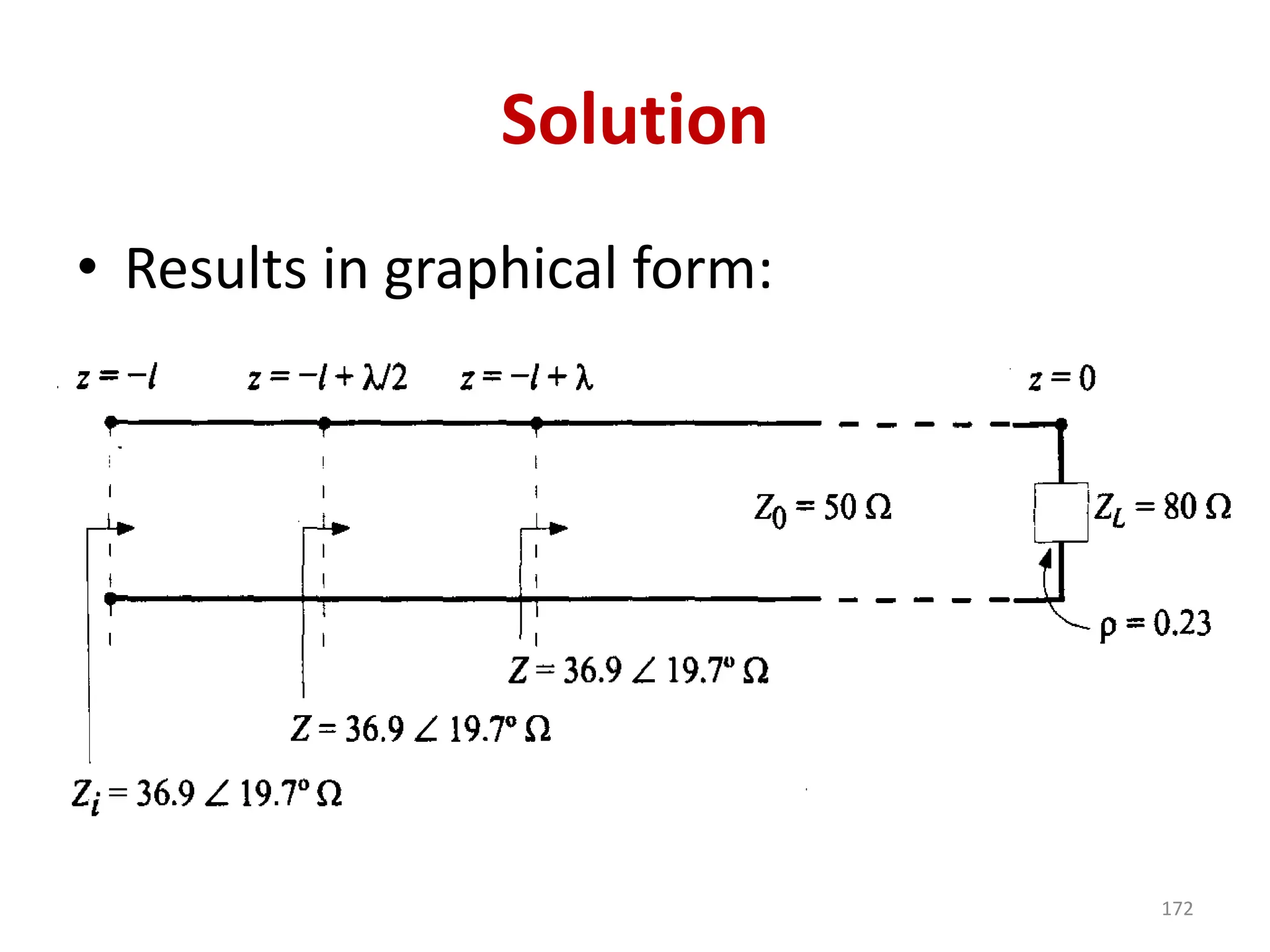
Solution
• The valuesof the three impedances are
equal due to the periodic nature of the
trigonometric functions involved in the
formulas.
• The value of Z is repeated every λ/2, instead
of every time λ is advanced, because in an
unmatched line the total wave that is formed
has a period equal to λ/2.
173
174.
Exercise 2.18.9 (fromthe book)
• A lossless coaxial cable with
characteristic impedance of 75 Ω
employs a dielectric with relative
permittivity of 2.26. The cable terminates
at a resistive load of 100 Ω and works at
a frequency of 600 MHz.
174
175.
Ejercicio 2.18.9 (Libro)
•Calculate the impedance seen at the
following points on the line: a) at the load, b)
at 10 cm before the load, c) at λ/4 before the
load, d) at λ/2 before the load, and e) at 3λ/2
before the load. [Z = 100 Ω, Z = 58.8 + j10.2
Ω, Z = 56.25 Ω, Z = 100 Ω, Z = 100 Ω].[Z = 100
Ω, Z = 58.8 + j10.2 Ω, Z = 56.25 Ω, Z = 100 Ω,
Z = 100 Ω].
175
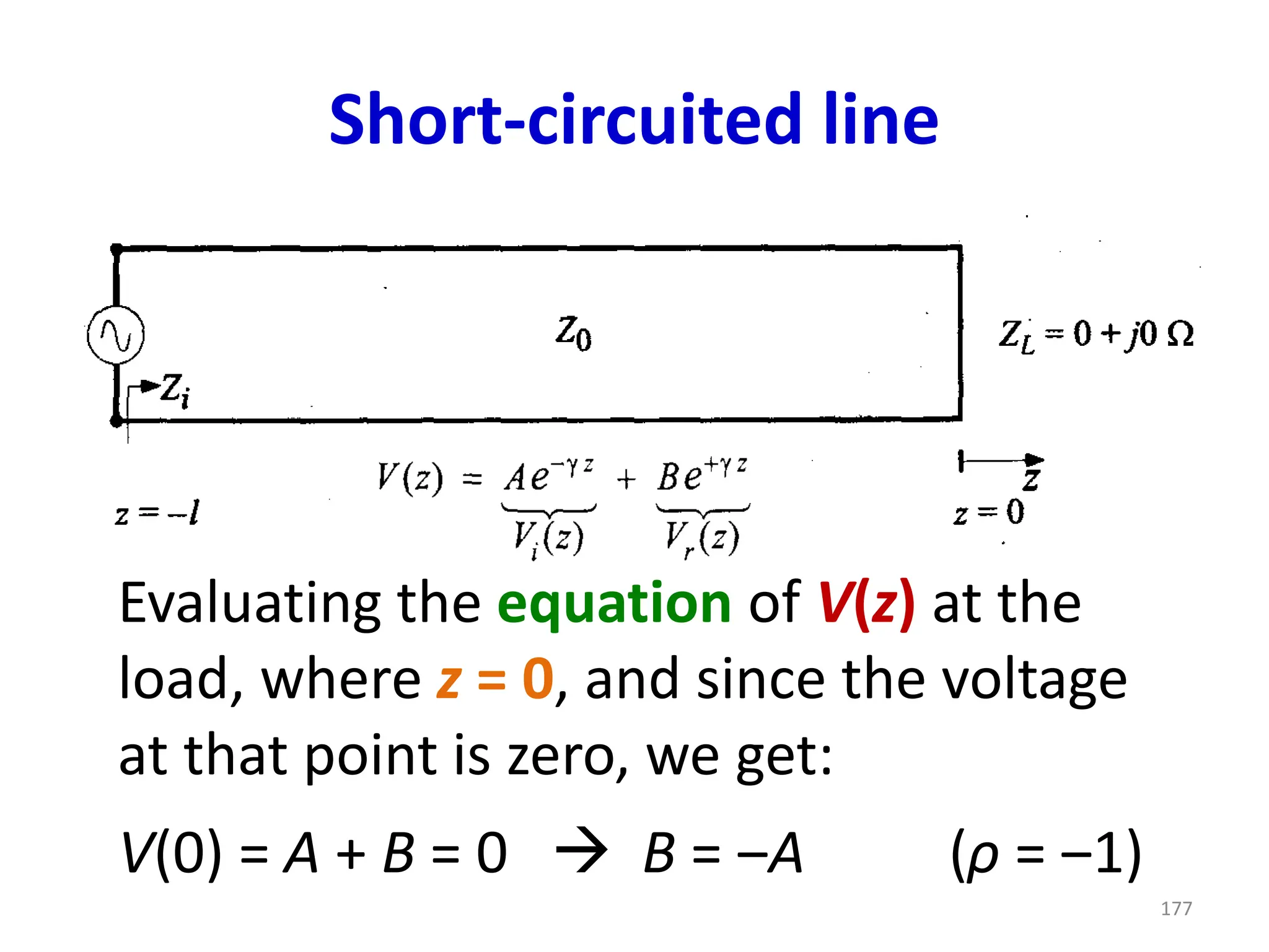
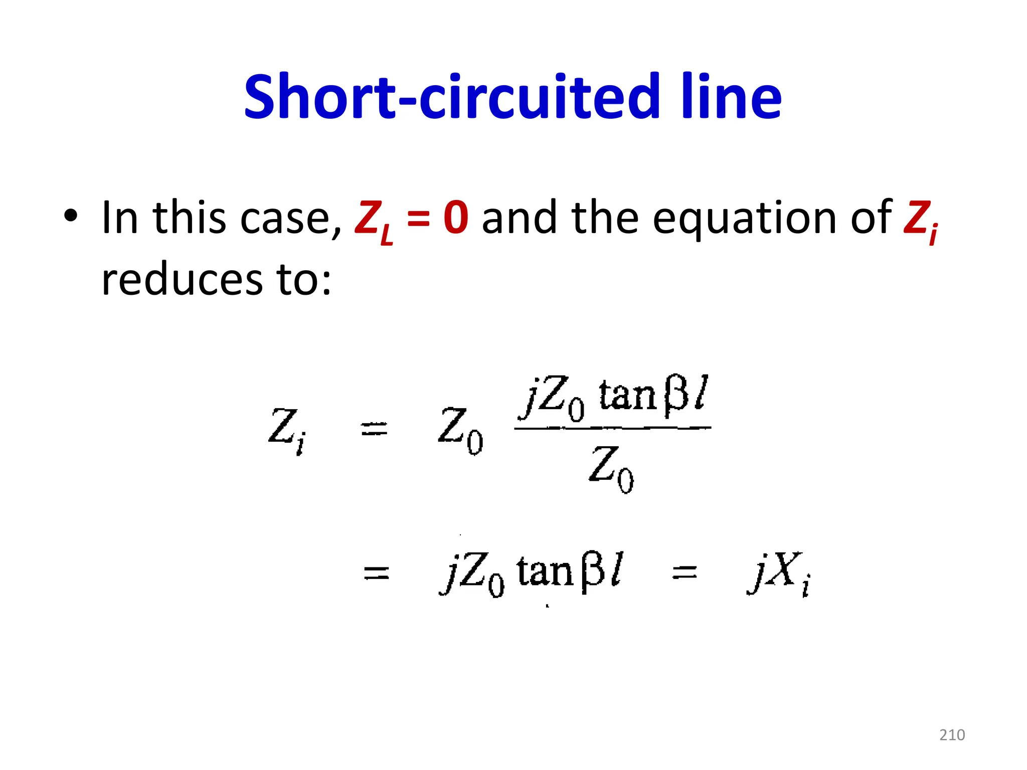
Short-circuited line
Evaluating theequation of V(z) at the
load, where z = 0, and since the voltage
at that point is zero, we get:
V(0) = A + B = 0 → B = ‒A (ρ = ‒1)
177
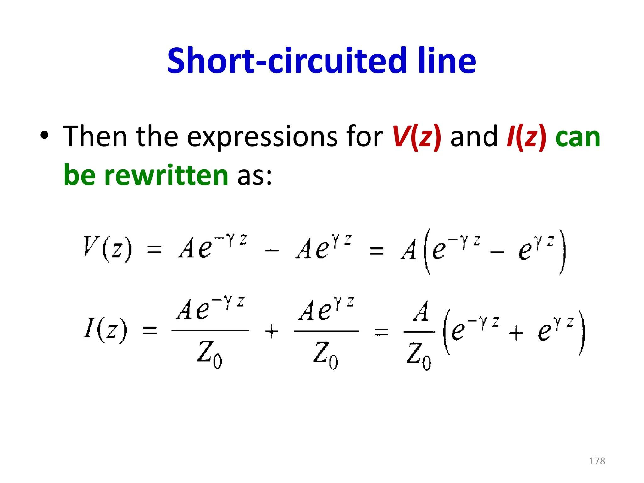
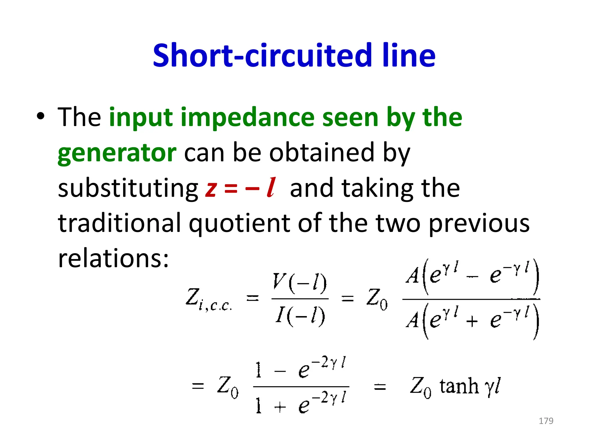
Short-circuited line
• Theinput impedance seen by the
generator can be obtained by
substituting z = ‒ l and taking the
traditional quotient of the two previous
relations:
179
180.
Short-circuited line
• Inpractice, measuring the input
impedance of a short-circuited line
makes it possible to indirectly
measure parameters R and L of the
line.
180
181.
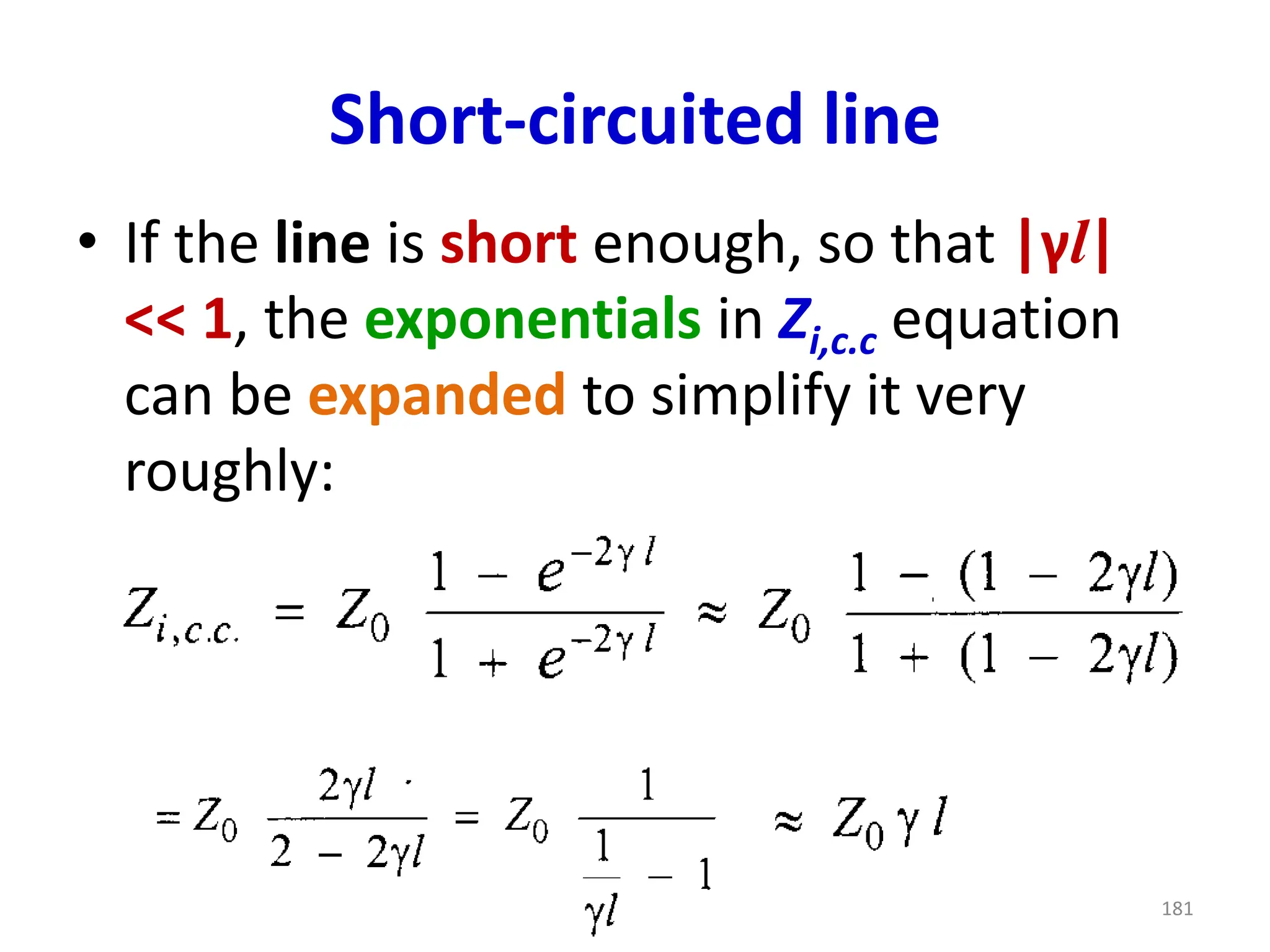
Short-circuited line
• Ifthe line is short enough, so that |γl|
<< 1, the exponentials in Zi,c.c equation
can be expanded to simplify it very
roughly:
181
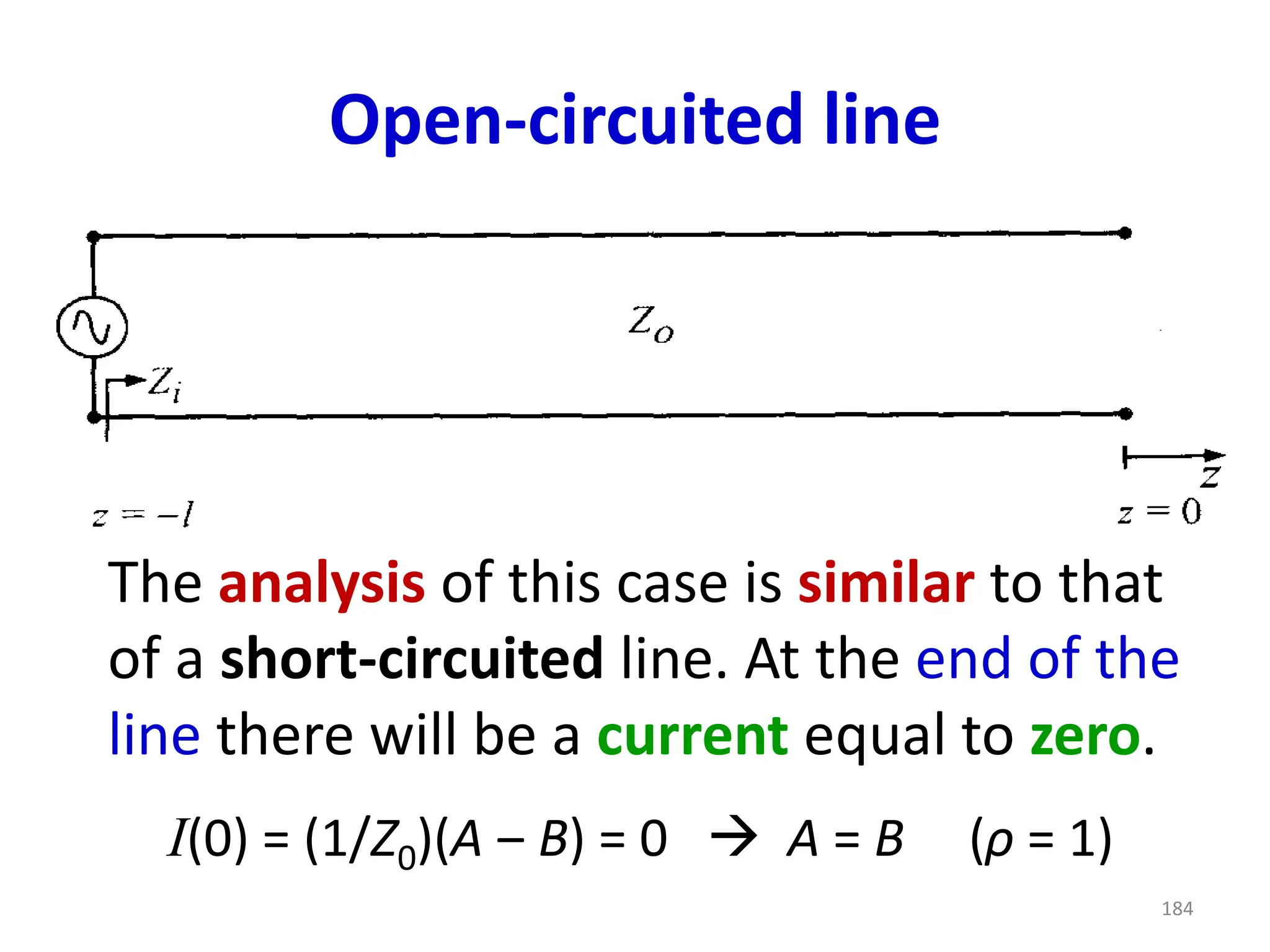
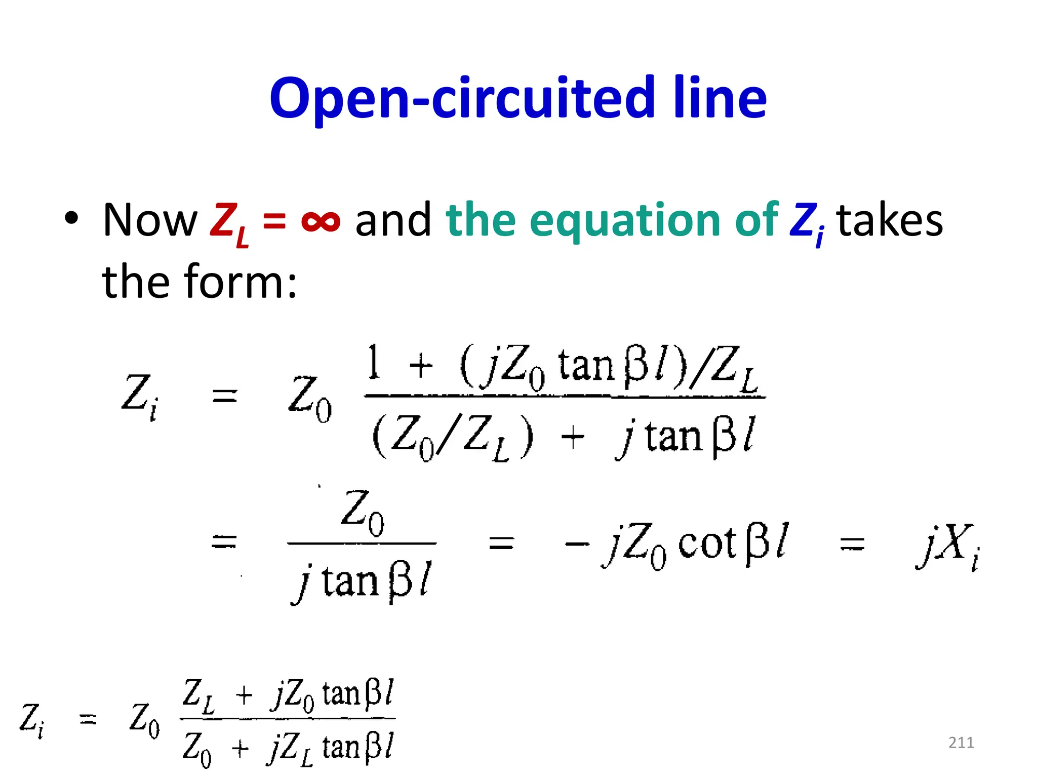
Open-circuited line
The analysisof this case is similar to that
of a short-circuited line. At the end of the
line there will be a current equal to zero.
I(0) = (1/Z0)(A ‒ B) = 0 → A = B (ρ = 1)
184
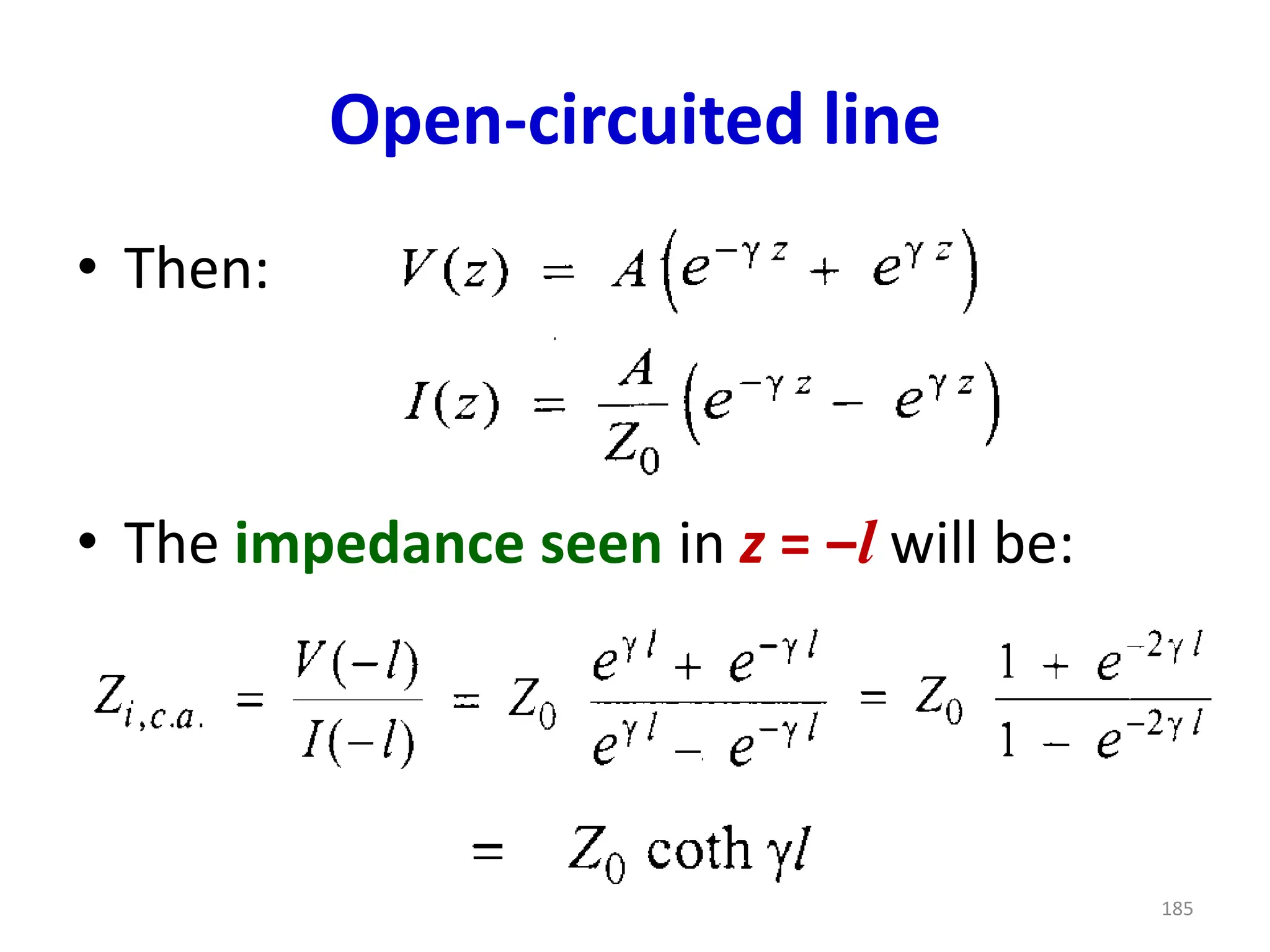
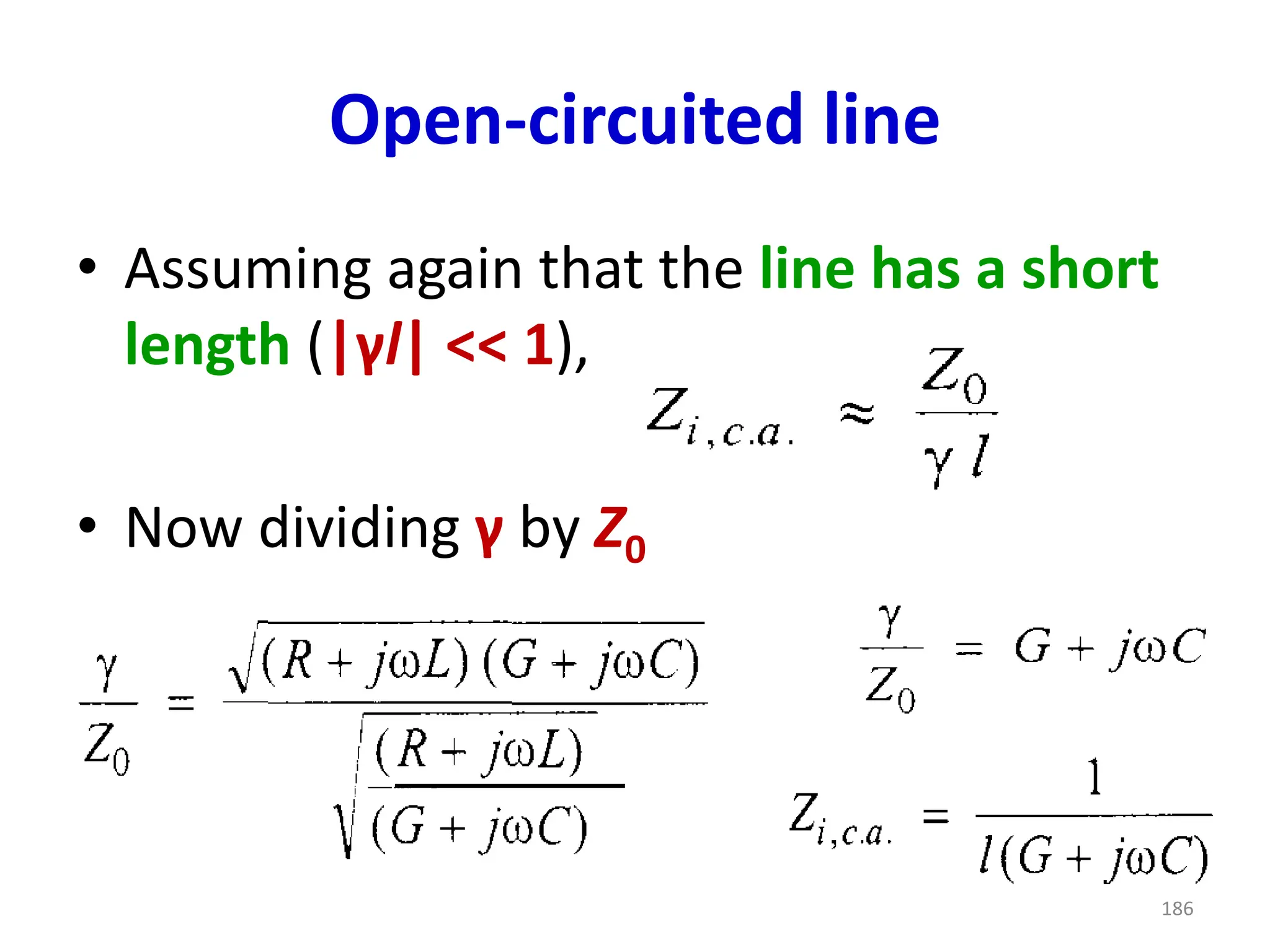
Open-circuited line
• Therefore,the input impedance
measured at a certain angular
frequency ω for an open-circuited
short line of length l, allows to
obtain the parameters G and C of the
line.
187
188.
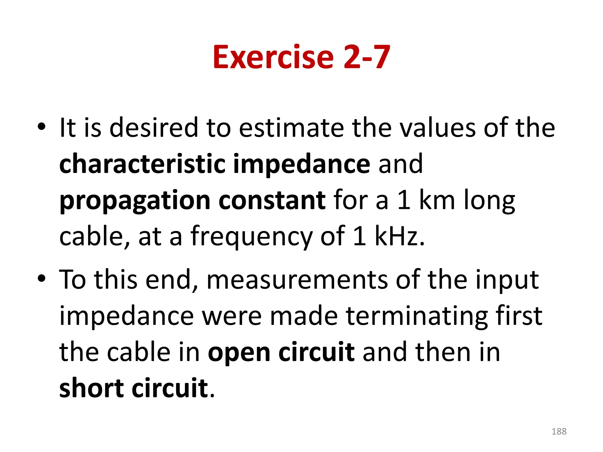
Exercise 2-7
• Itis desired to estimate the values of the
characteristic impedance and
propagation constant for a 1 km long
cable, at a frequency of 1 kHz.
• To this end, measurements of the input
impedance were made terminating first
the cable in open circuit and then in
short circuit.
188
189.
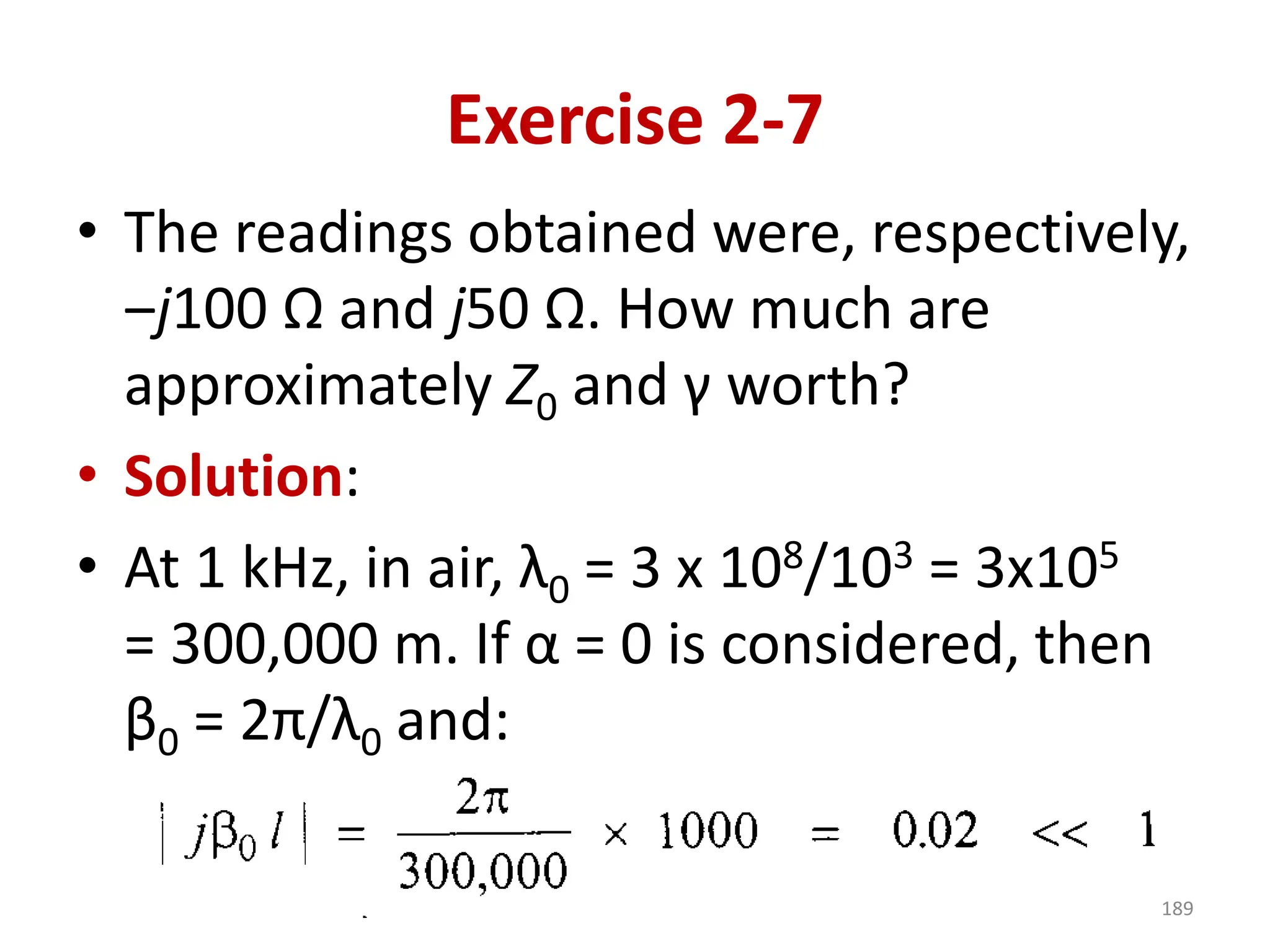
Exercise 2-7
• Thereadings obtained were, respectively,
‒j100 Ω and j50 Ω. How much are
approximately Z0 and γ worth?
• Solution:
• At 1 kHz, in air, λ0 = 3 x 10⁸/103 = 3x105
= 300,000 m. If α = 0 is considered, then
β0 = 2π/λ0 and:
189
190.
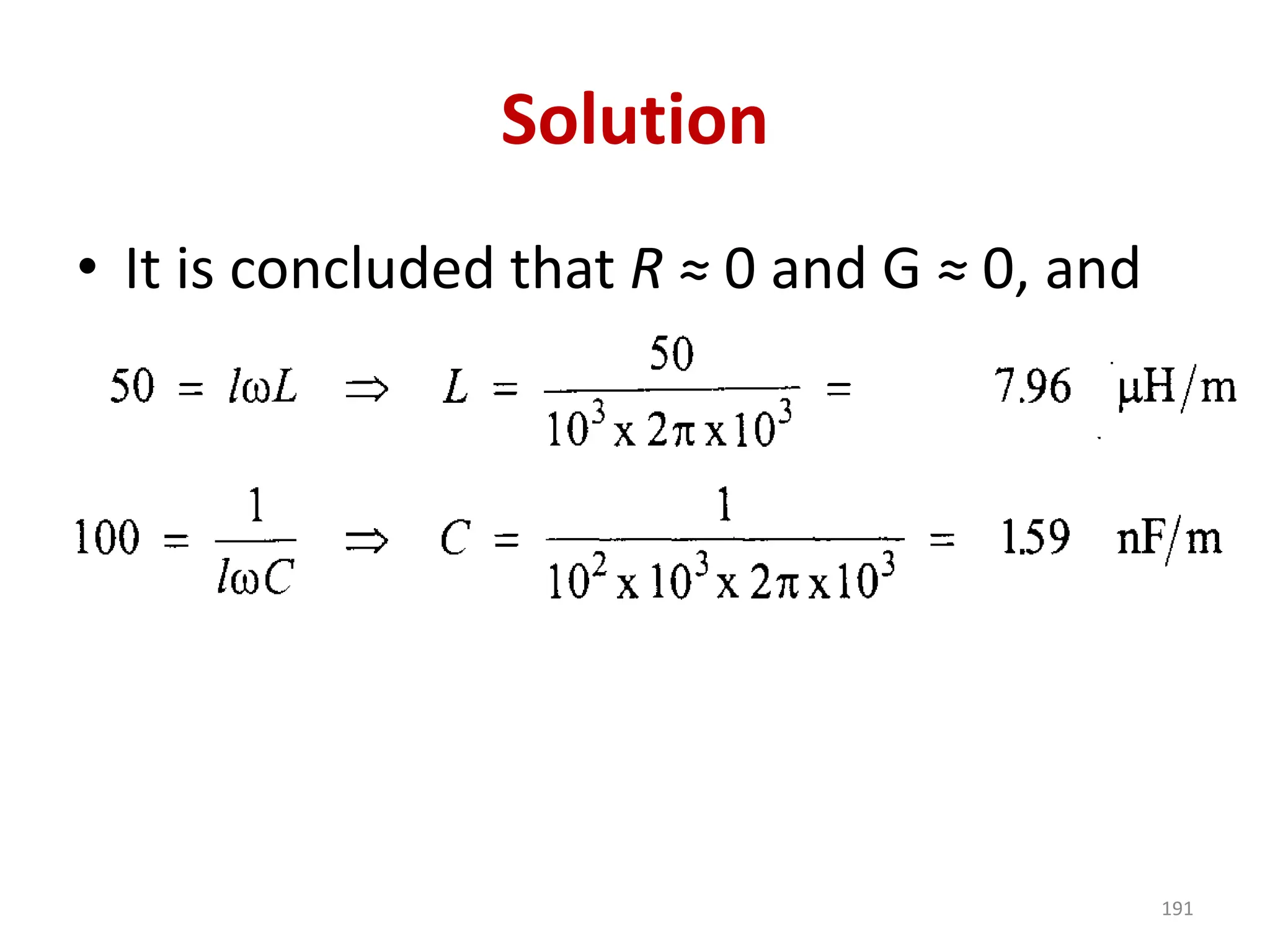
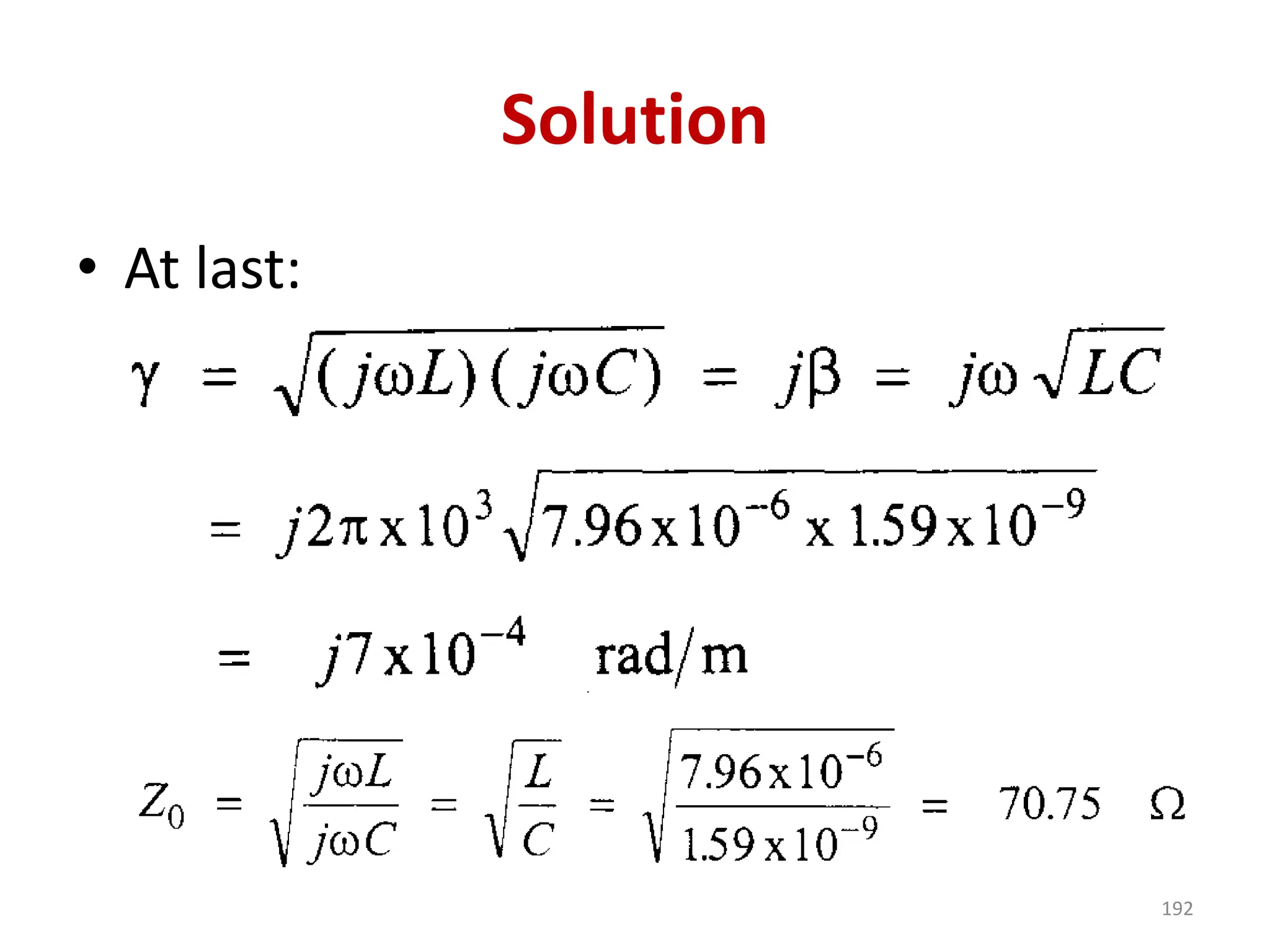
Solution
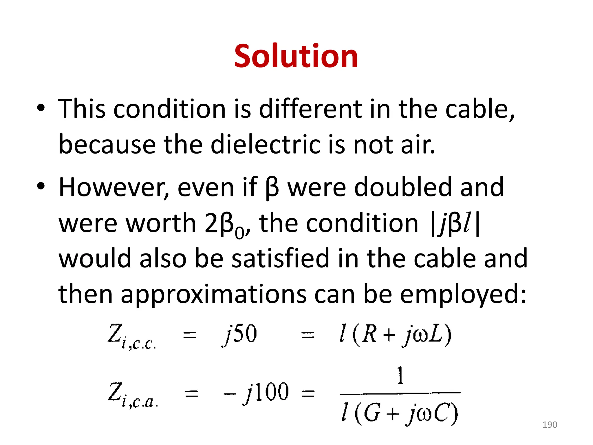
• This conditionis different in the cable,
because the dielectric is not air.
• However, even if β were doubled and
were worth 2β0, the condition |jβl|
would also be satisfied in the cable and
then approximations can be employed:
190
Obtaining Z0 frominput
impedances measured on
short-circuited and open-
circuited lines.
194.
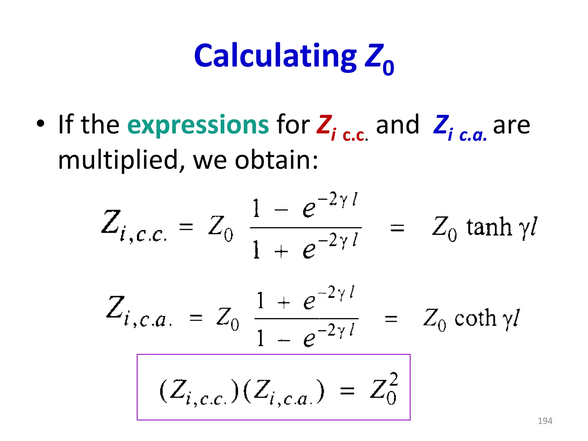
Calculating Z0
• Ifthe expressions for Zi c.c. and Zi c.a. are
multiplied, we obtain:
194
195.
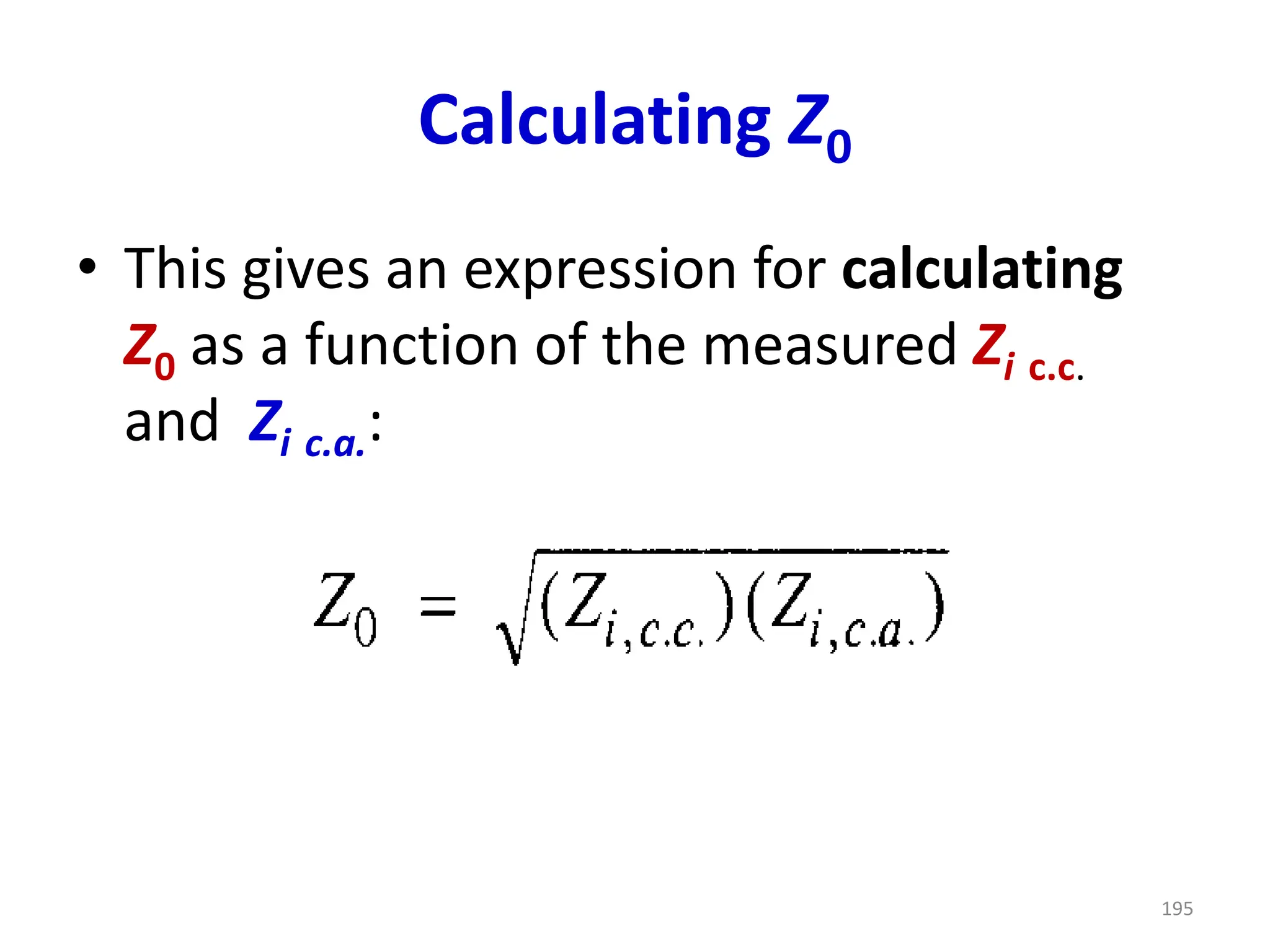
Calculating Z0
• Thisgives an expression for calculating
Z0 as a function of the measured Zi c.c.
and Zi c.a.:
195
196.
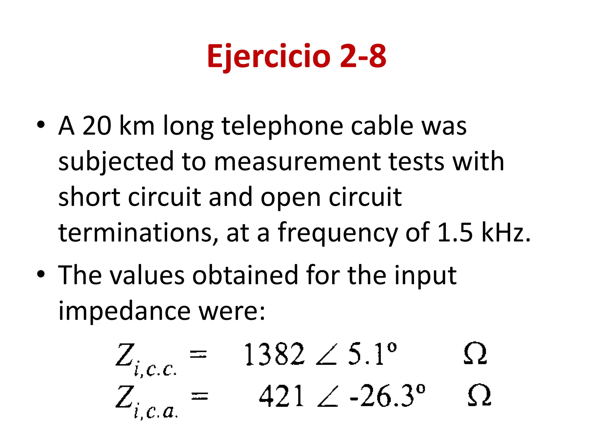
Ejercicio 2-8
• A20 km long telephone cable was
subjected to measurement tests with
short circuit and open circuit
terminations, at a frequency of 1.5 kHz.
• The values obtained for the input
impedance were:
197.
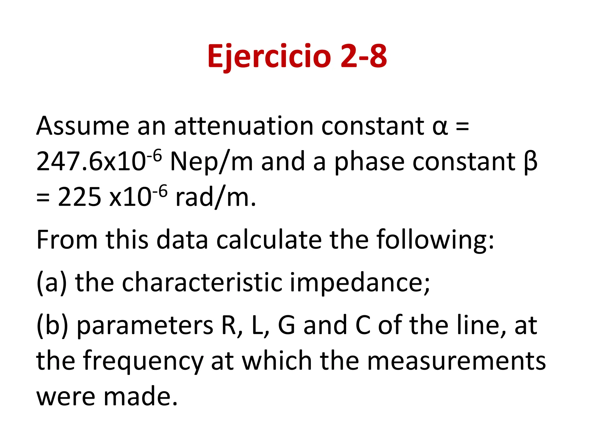
Ejercicio 2-8
Assume anattenuation constant α =
247.6x10⁻⁶ Nep/m and a phase constant β
= 225 x10-6 rad/m.
From this data calculate the following:
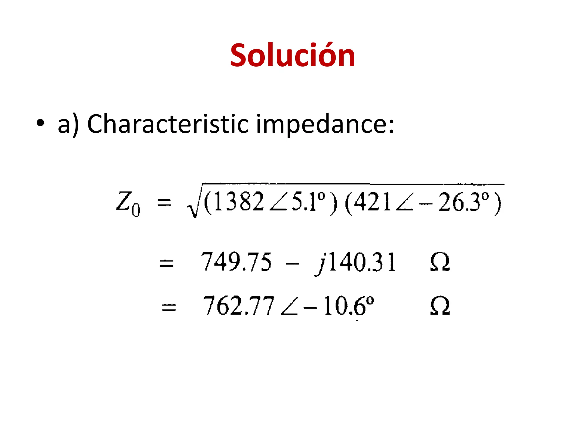
(a) the characteristic impedance;
(b) parameters R, L, G and C of the line, at
the frequency at which the measurements
were made.
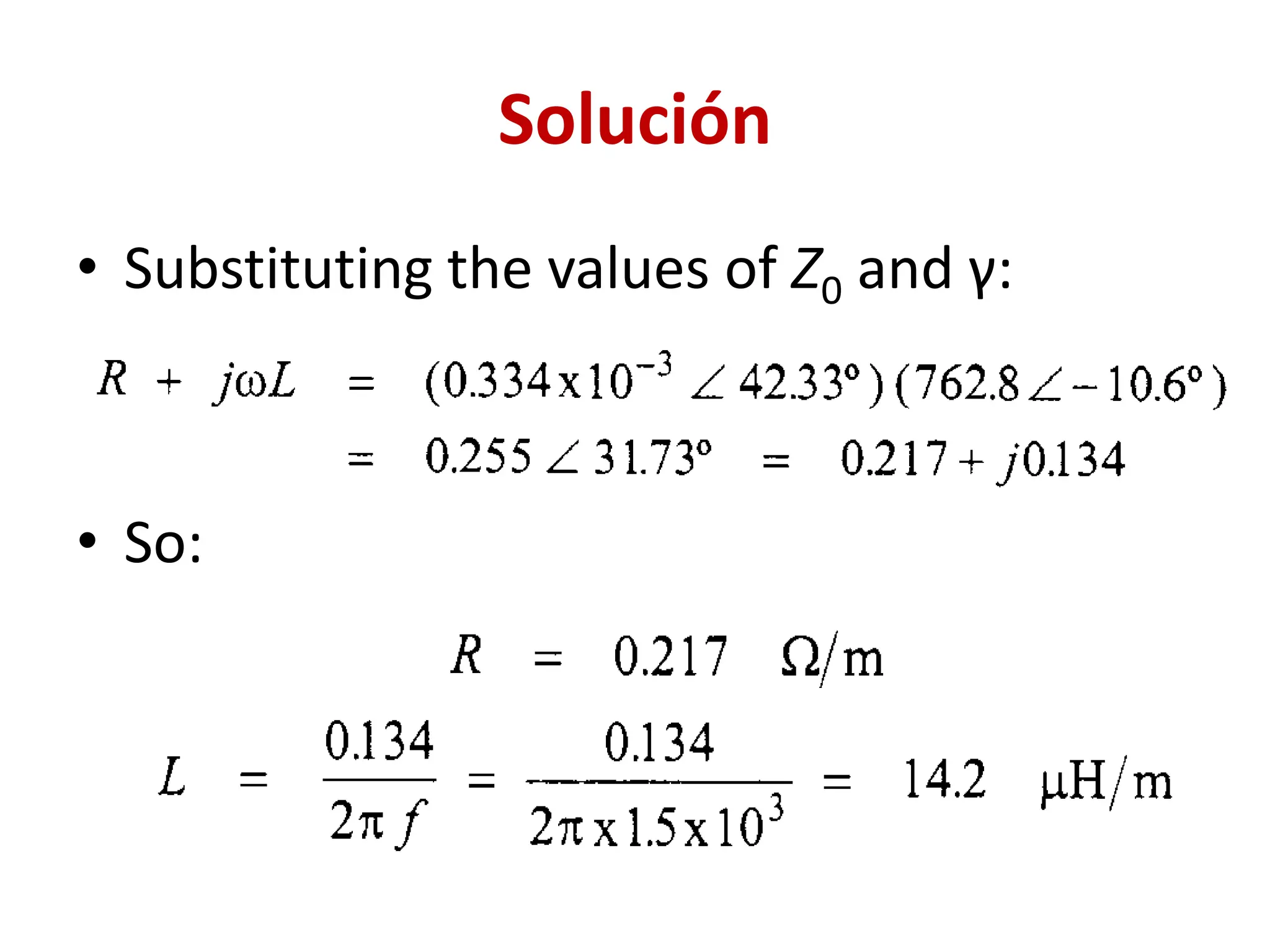
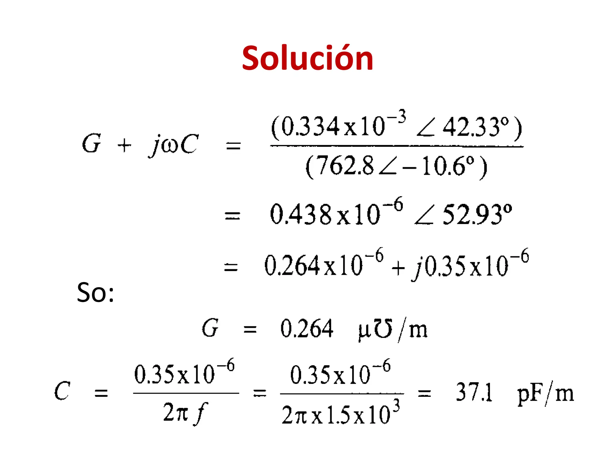
Solución
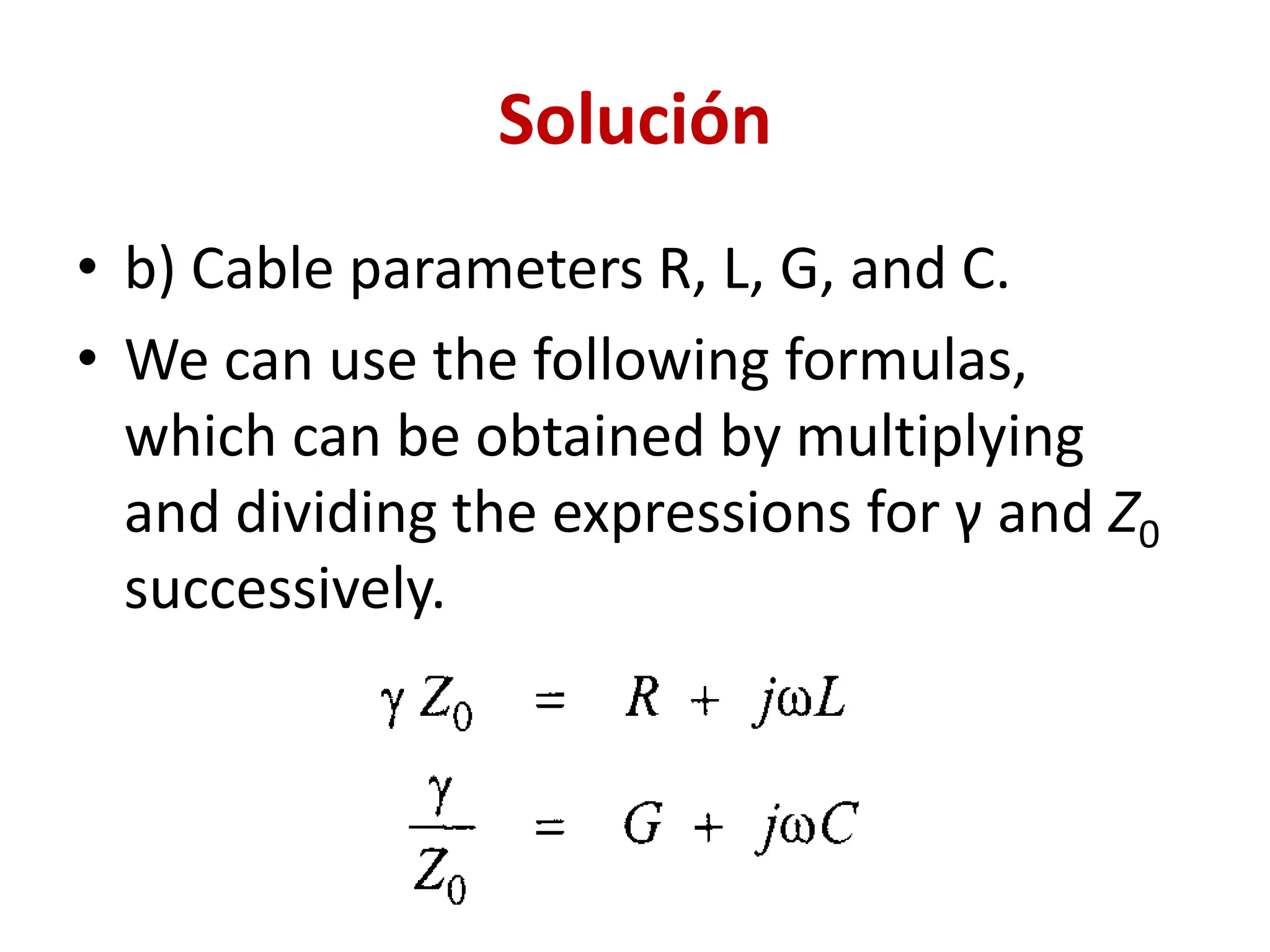
• b) Cableparameters R, L, G, and C.
• We can use the following formulas,
which can be obtained by multiplying
and dividing the expressions for γ and Z0
successively.
Input reactance andshort-
circuited and open-circuited
lossless line applications
203.
Introduction
• In additionto being used to transmit
information, a line can also serve as
a circuit element.
• At UHF (300 MHz to 3 GHz) it is
difficult to fabricate circuit elements
with concentrated parameters, as
the λ varies between 10 cm and 1 m.
203
204.
Introduction
• For thesecases, transmission line
segments can be designed to
produce an inductive or capacitive
impedance, which can be used to
match an arbitrary load to the main
line and achieve the maximum
possible power transfer.
204
205.
Introduction
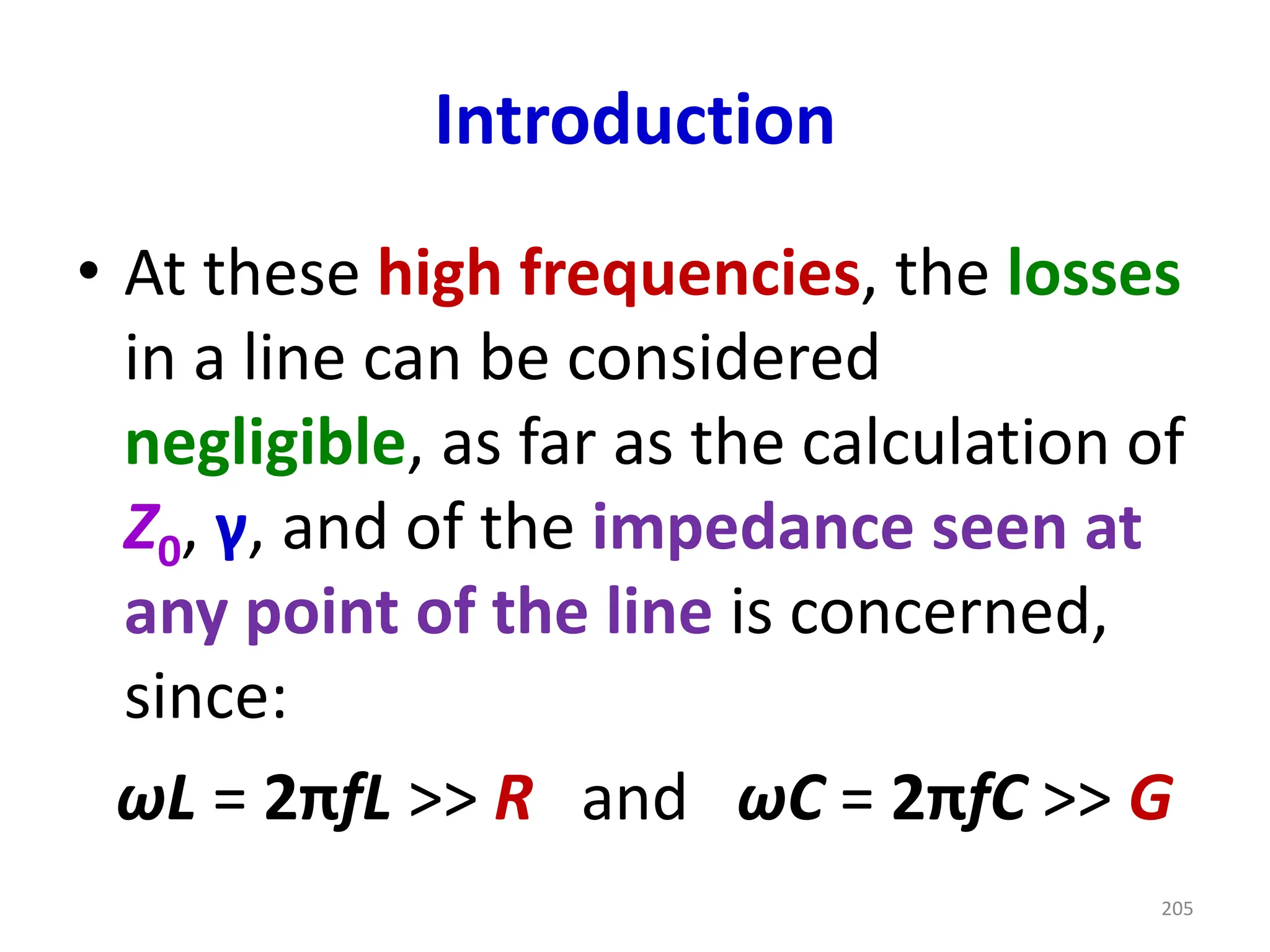
• At thesehigh frequencies, the losses
in a line can be considered
negligible, as far as the calculation of
Z0, γ, and of the impedance seen at
any point of the line is concerned,
since:
ωL = 2πfL >> R and ωC = 2πfC >> G
205
206.
Z0 and γ
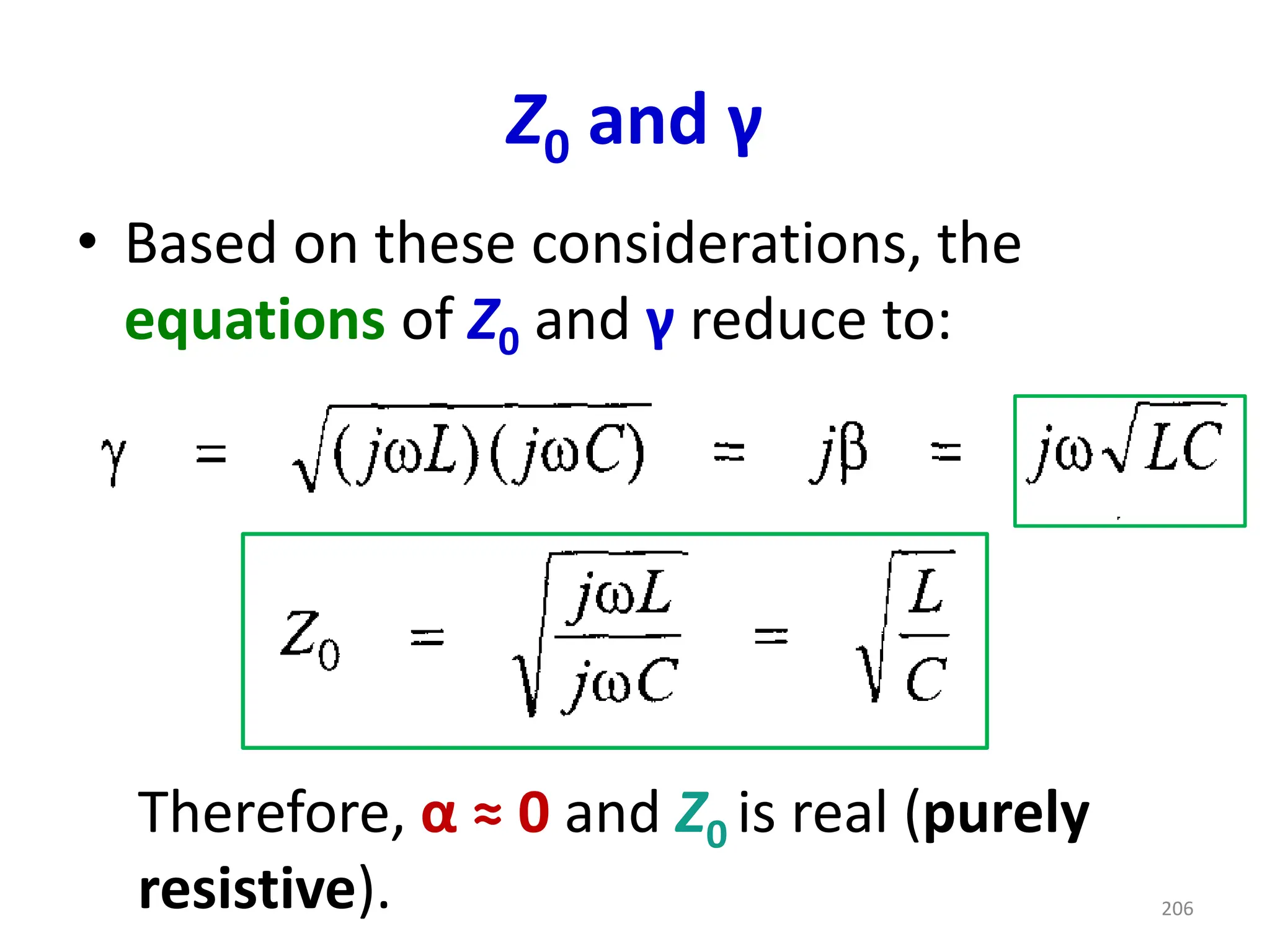
•Based on these considerations, the
equations of Z0 and γ reduce to:
Therefore, α ≈ 0 and Z0 is real (purely
resistive). 206
207.
Input impedance
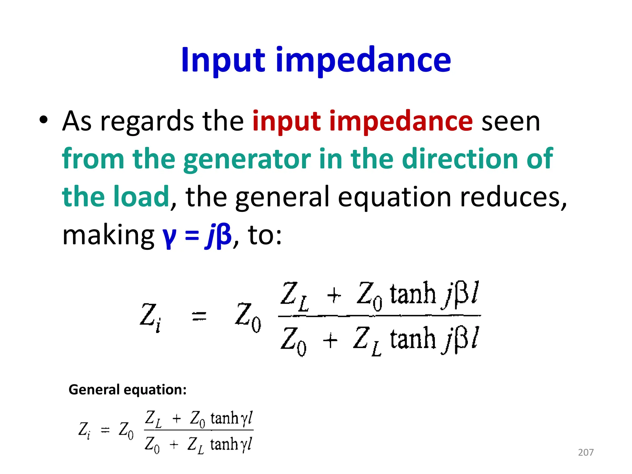
• Asregards the input impedance seen
from the generator in the direction of
the load, the general equation reduces,
making γ = jβ, to:
General equation:
207
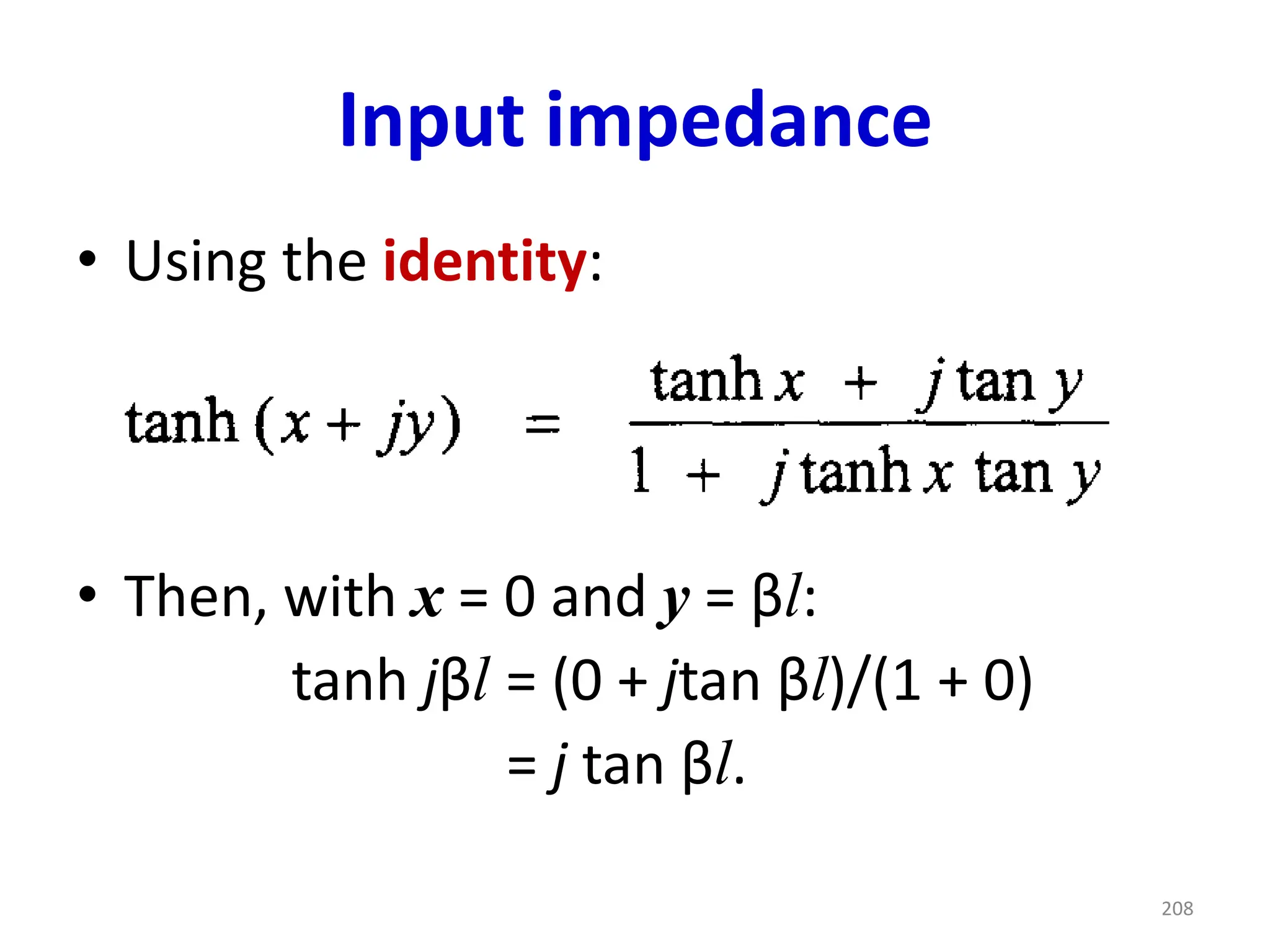
208.
Input impedance
• Usingthe identity:
• Then, with x = 0 and y = βl:
tanh jβl = (0 + jtan βl)/(1 + 0)
= j tan βl.
208
209.
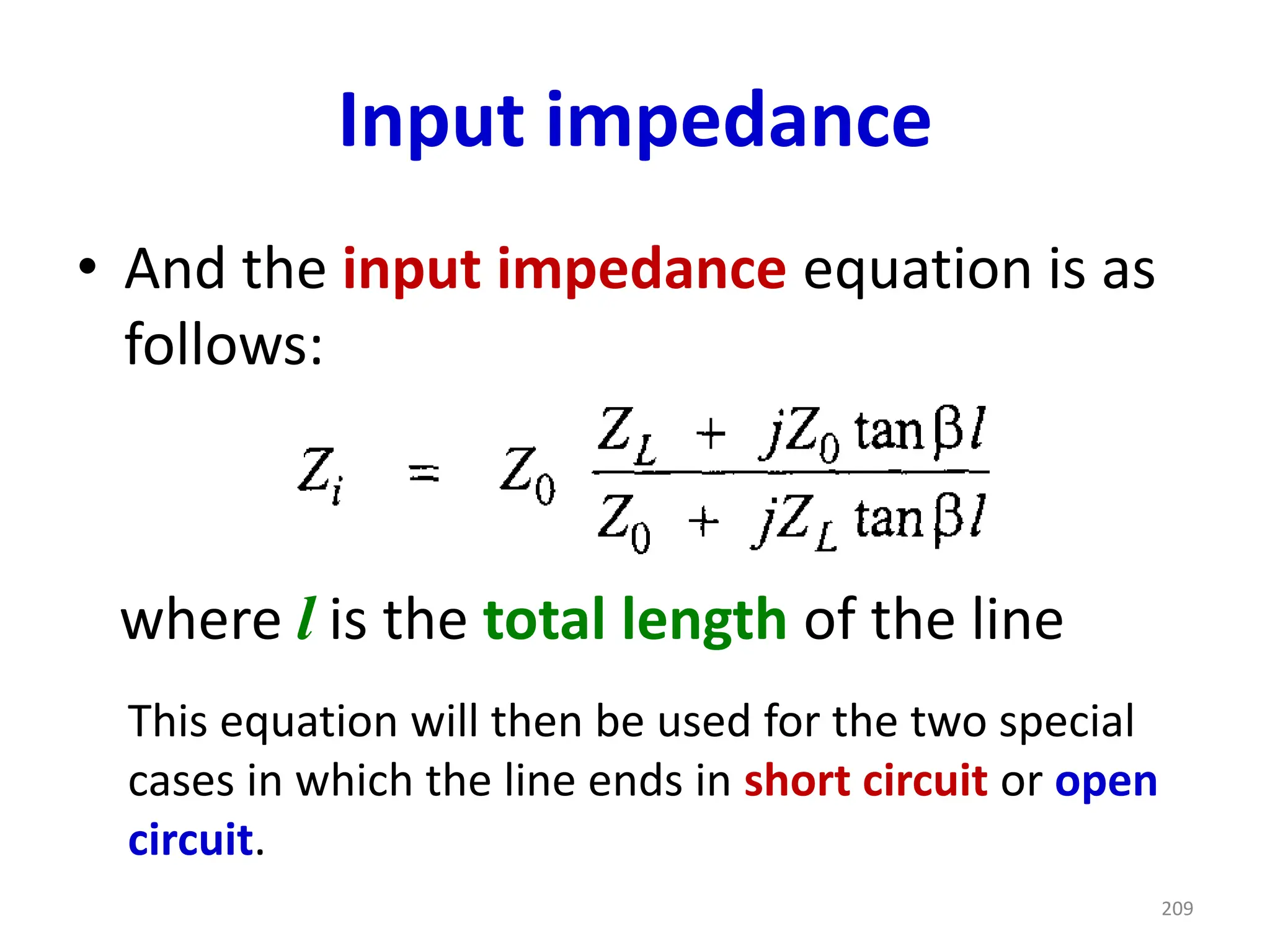
Input impedance
• Andthe input impedance equation is as
follows:
where l is the total length of the line
This equation will then be used for the two special
cases in which the line ends in short circuit or open
circuit.
209
Input reactance
• Theabove Zi equations show that
when a lossless line of arbitrary
length l is short-circuited or open-
circuited, the input impedance is
purely reactive (jXi).
212
213.
Input reactance
• Ineither case, the reactance can be
inductive or capacitive, depending
on the value of βl, since the
functions tan(βl) and cot(βl) can take
positive or negative values.
213
214.
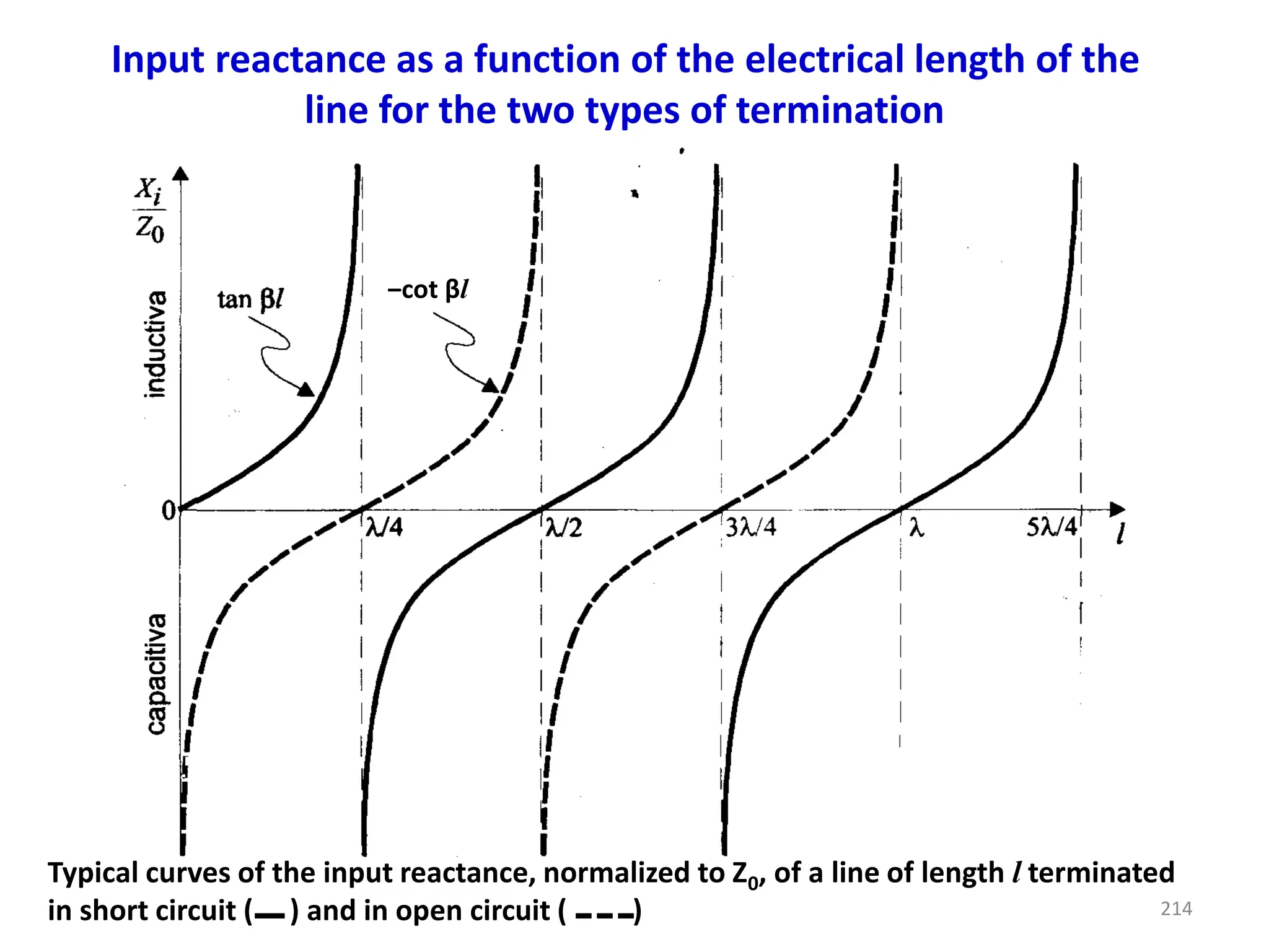
Input reactance asa function of the electrical length of the
line for the two types of termination
Typical curves of the input reactance, normalized to Z0, of a line of length l terminated
in short circuit ( ) and in open circuit ( )
‒cot βl
214
215.
Input reactance
• Inpractice, it is not possible to
obtain a truly open-circuited line
(infinite load impedance), since
there are radiation problems at the
open end, especially at high
frequencies, and coupling with
nearby objects.
215
216.
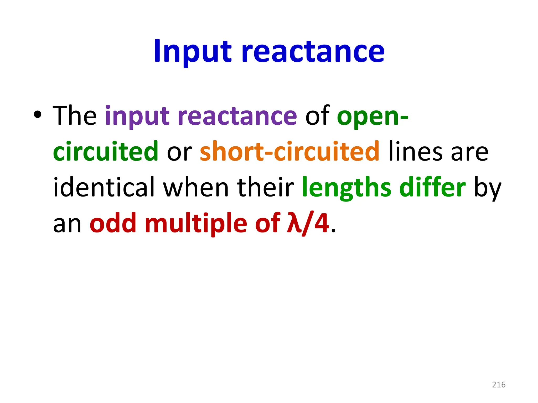
Input reactance
• Theinput reactance of open-
circuited or short-circuited lines are
identical when their lengths differ by
an odd multiple of λ/4.
216
217.
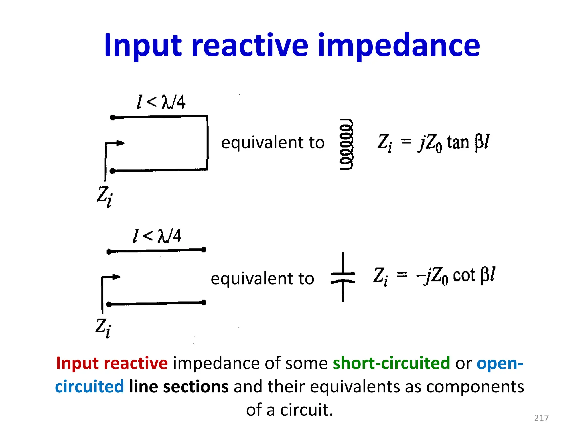
Input reactive impedance
Inputreactive impedance of some short-circuited or open-
circuited line sections and their equivalents as components
of a circuit. 217
equivalent to
equivalent to
218.
Input reactive impedance
218
equivalentto
equivalent to
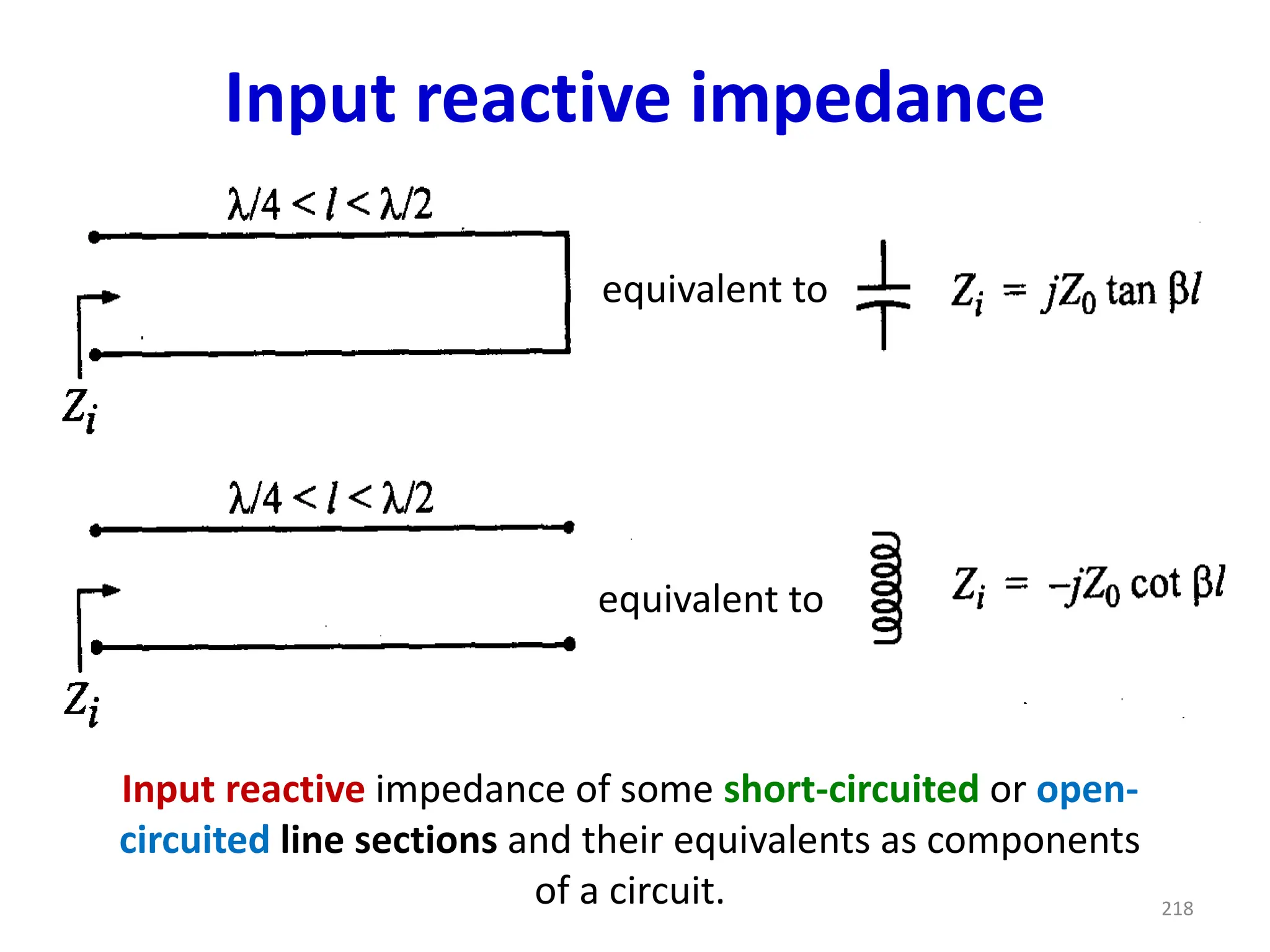
Input reactive impedance of some short-circuited or open-
circuited line sections and their equivalents as components
of a circuit.
219.
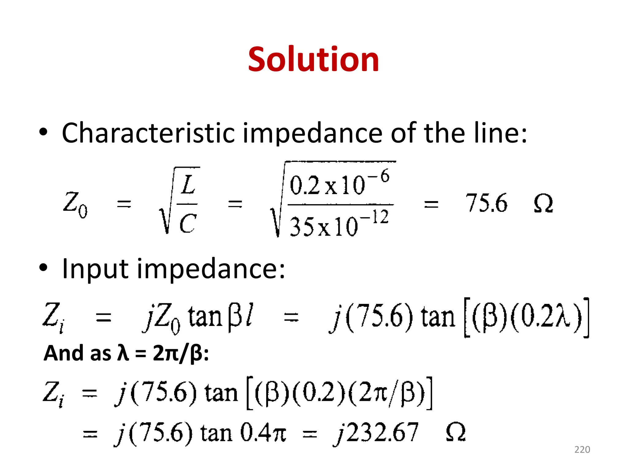
Exercise 2-9
• Considera lossless line of length 0.2λ at a
certain operating frequency terminated
in short circuit.
• Its L and C parameters are 0.2 μH/m and
35 pF/m, respectively. Calculate its input
impedance.
219
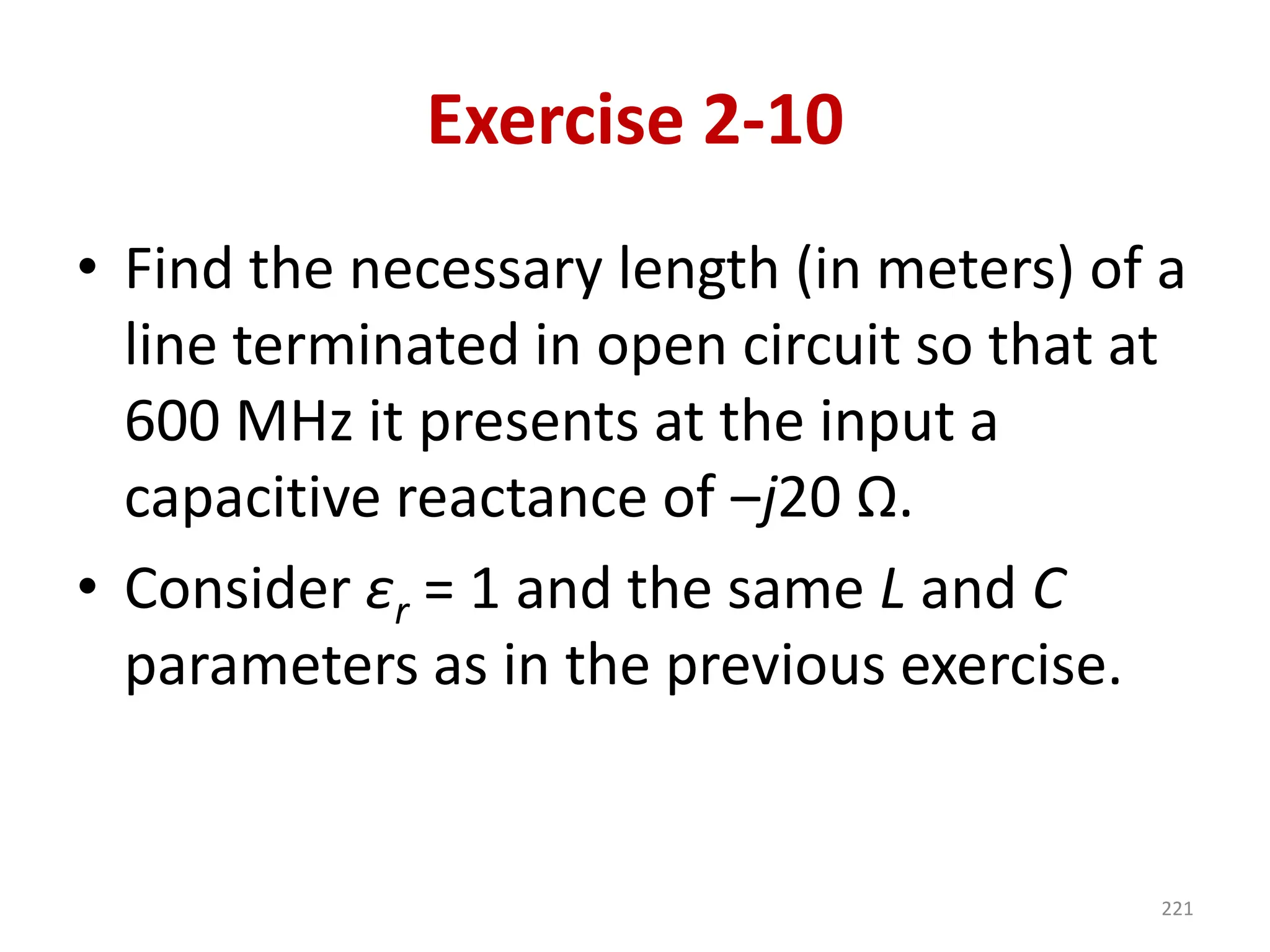
Exercise 2-10
• Findthe necessary length (in meters) of a
line terminated in open circuit so that at
600 MHz it presents at the input a
capacitive reactance of ‒j20 Ω.
• Consider εr = 1 and the same L and C
parameters as in the previous exercise.
221
222.
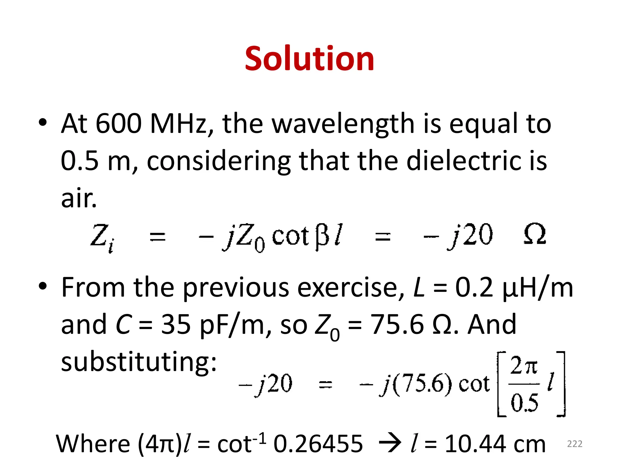
Solution
• At 600MHz, the wavelength is equal to
0.5 m, considering that the dielectric is
air.
• From the previous exercise, L = 0.2 μH/m
and C = 35 pF/m, so Z0 = 75.6 Ω. And
substituting:
Where (4π)l = cot-1 0.26455 → l = 10.44 cm 222
223.
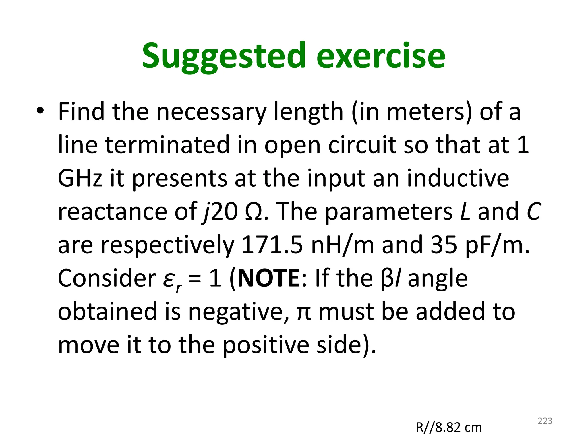
Suggested exercise
• Findthe necessary length (in meters) of a
line terminated in open circuit so that at 1
GHz it presents at the input an inductive
reactance of j20 Ω. The parameters L and C
are respectively 171.5 nH/m and 35 pF/m.
Consider εr = 1 (NOTE: If the βl angle
obtained is negative, π must be added to
move it to the positive side).
223
R//8.82 cm
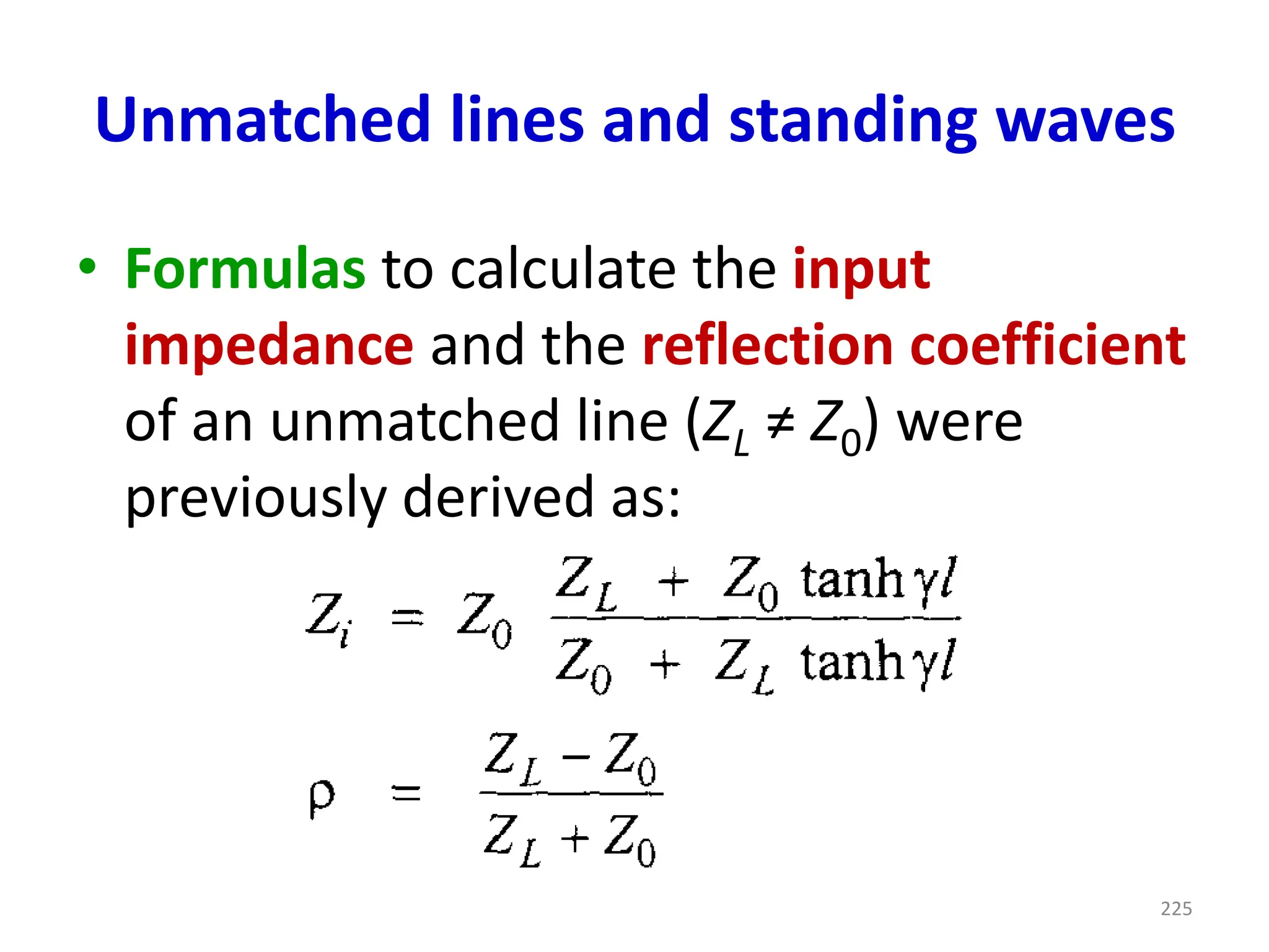
Unmatched lines andstanding waves
• Formulas to calculate the input
impedance and the reflection coefficient
of an unmatched line (ZL ≠ Z0) were
previously derived as:
225
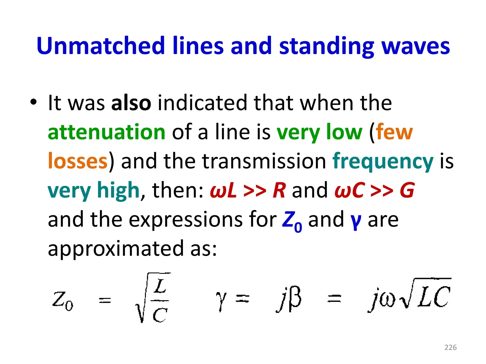
226.
Unmatched lines andstanding waves
• It was also indicated that when the
attenuation of a line is very low (few
losses) and the transmission frequency is
very high, then: ωL >> R and ωC >> G
and the expressions for Z0 and γ are
approximated as:
226
227.
Unmatched lines andstanding waves
• Henceforth, unless otherwise stated, it
will be assumed that α = 0 and that it is
transmitted at high frequencies.
• This approximation is valid in practice,
when l (length of the line) is, at most, a
few λ's and the accumulated attenuation
is very low.
227
228.
Unmatched lines andstanding waves
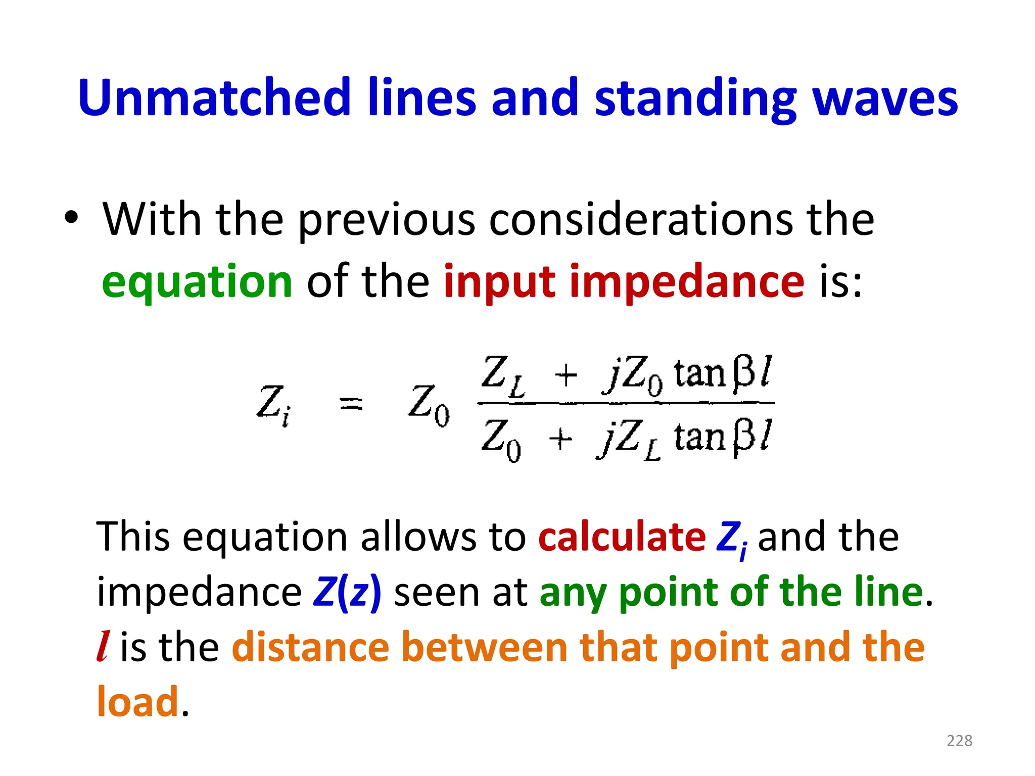
• With the previous considerations the
equation of the input impedance is:
This equation allows to calculate Zi and the
impedance Z(z) seen at any point of the line.
l is the distance between that point and the
load.
228
229.
Unmatched lines andstanding waves
• If ρ = 0, → matched line (ZL = Z0).
• If ρ ≠ 0, → unmatched line (ZL ≠ Z0).
• The goal of a transmission engineer is to
make ρ very small so that the power
transferred to the load is maximum.
229
230.
Unmatched lines andstanding waves
• Generally, a "coupling" is considered
acceptable if |ρ| ≤ 0.2, which delivers to
the load about 96% of the incident
power.
• We will now see what the total voltage
wave is like along an unmatched line.
230
231.
Unmatched lines andstanding waves
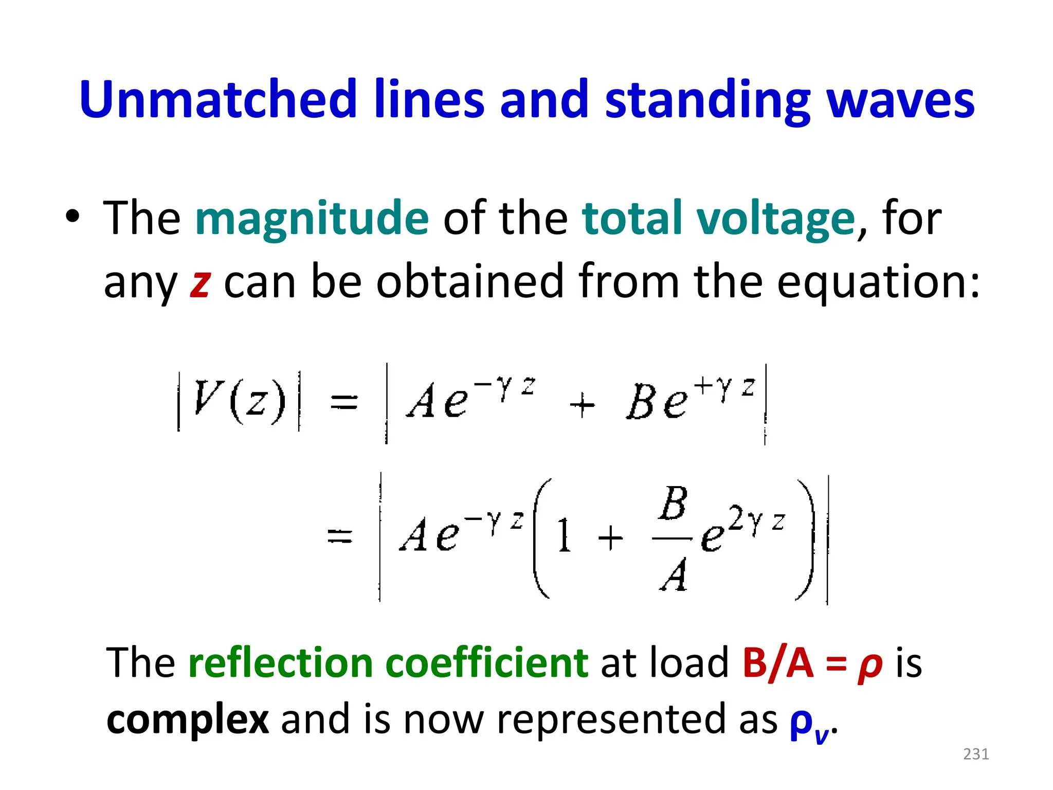
• The magnitude of the total voltage, for
any z can be obtained from the equation:
The reflection coefficient at load B/A = ρ is
complex and is now represented as ρv.
231
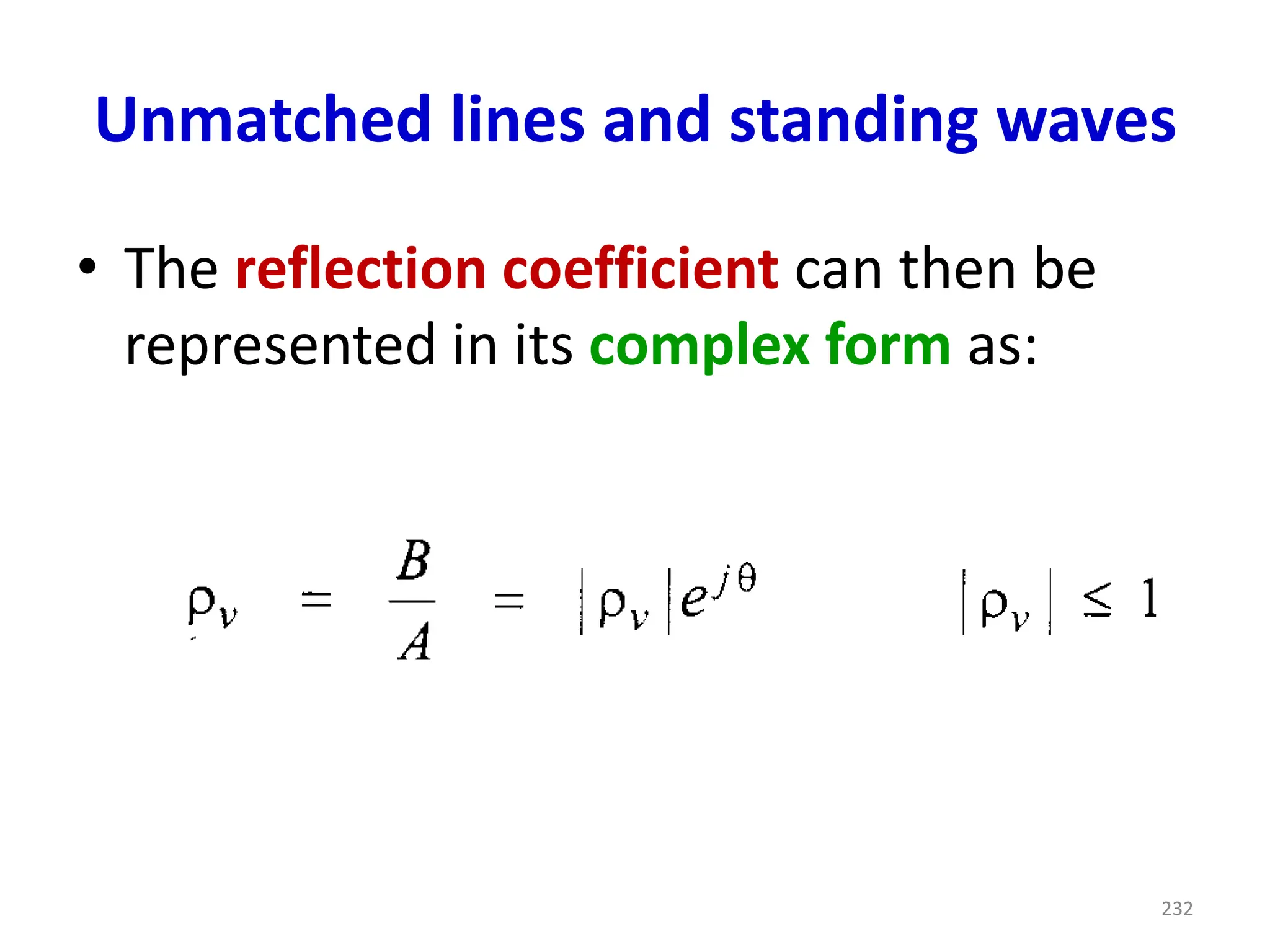
232.
Unmatched lines andstanding waves
• The reflection coefficient can then be
represented in its complex form as:
232
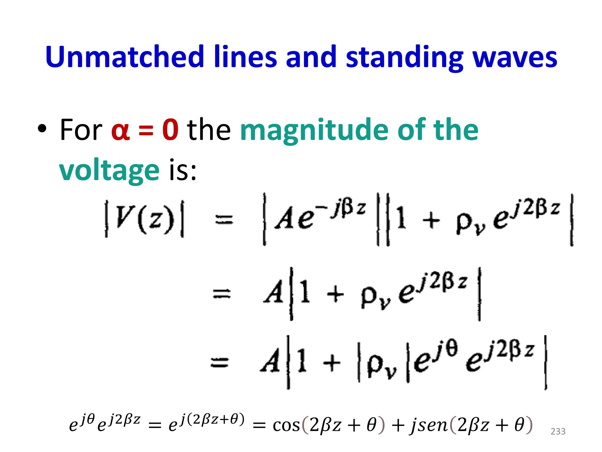
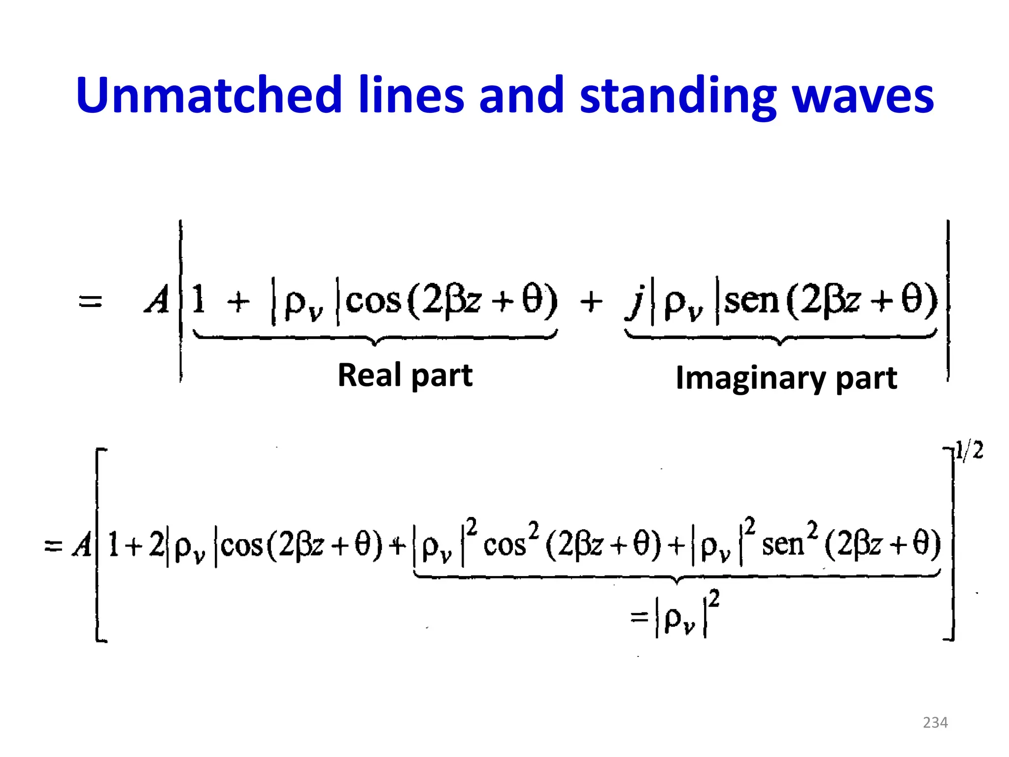
233.
Unmatched lines andstanding waves
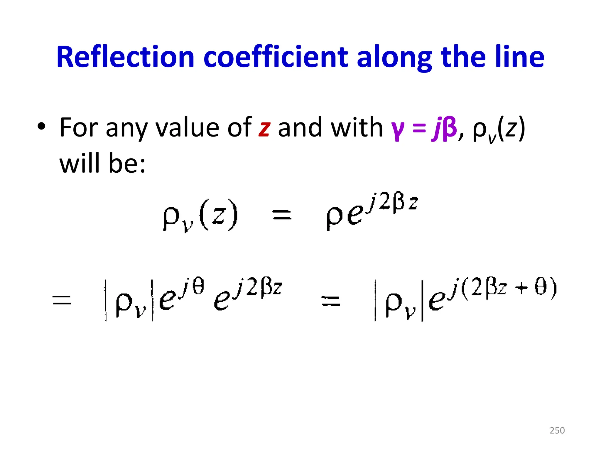
• For α = 0 the magnitude of the
voltage is:
233
𝑒𝑗𝜃𝑒𝑗2𝛽𝑧 = 𝑒𝑗 2𝛽𝑧+𝜃 = cos 2𝛽𝑧 + 𝜃 + 𝑗𝑠𝑒𝑛 2𝛽𝑧 + 𝜃
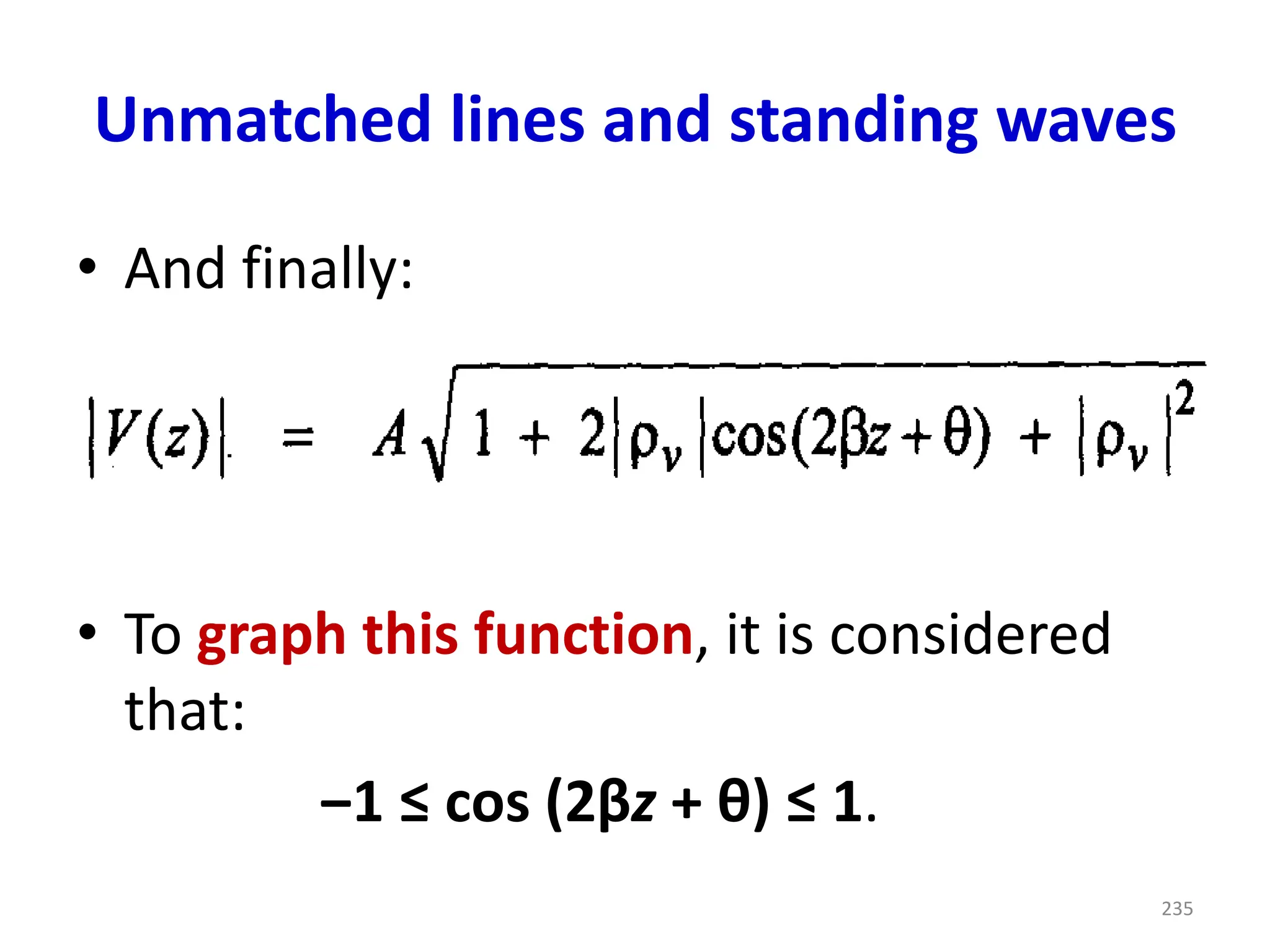
Unmatched lines andstanding waves
• And finally:
• To graph this function, it is considered
that:
‒1 ≤ cos (2βz + θ) ≤ 1.
235
236.
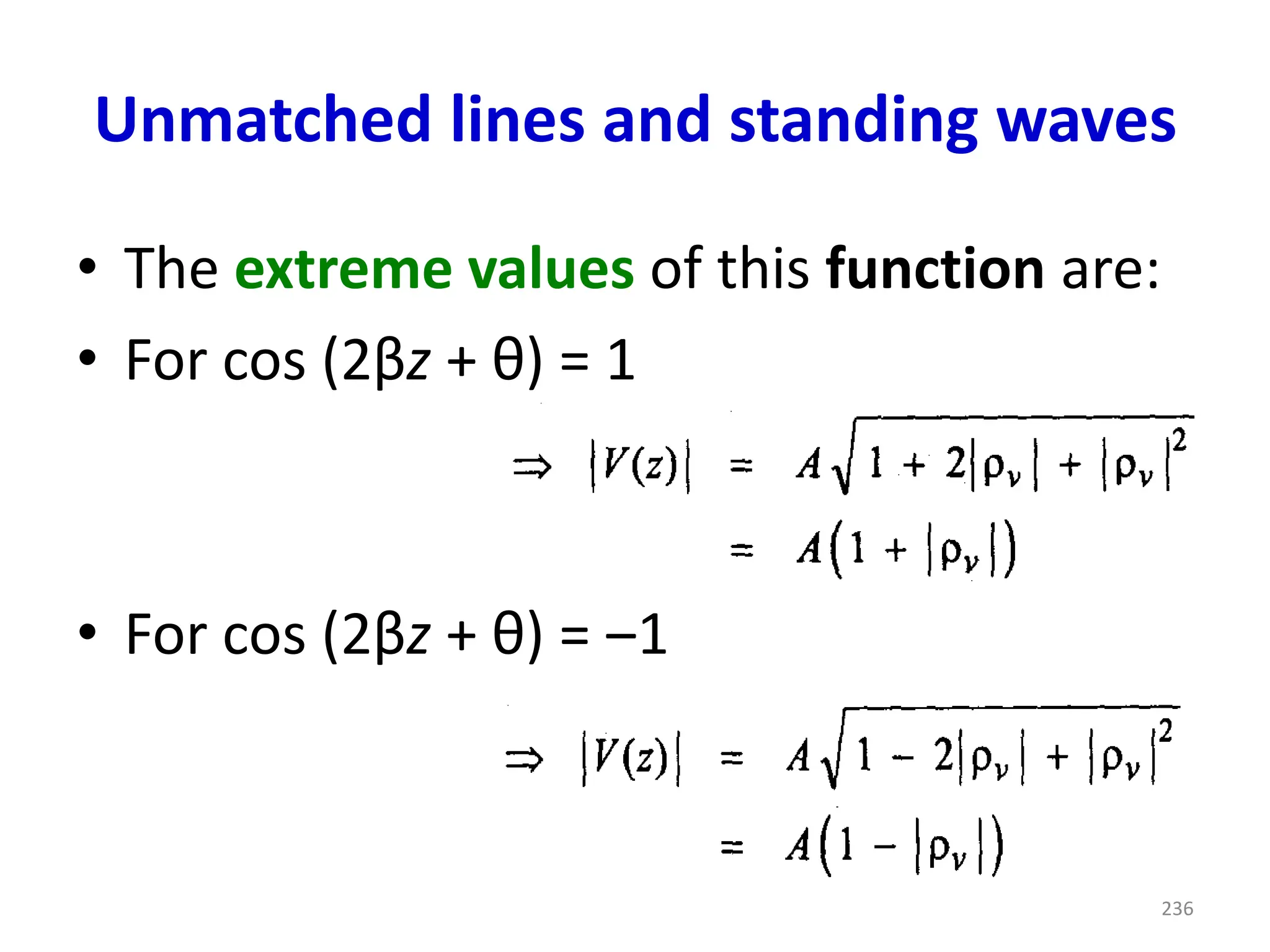
Unmatched lines andstanding waves
• The extreme values of this function are:
• For cos (2βz + θ) = 1
• For cos (2βz + θ) = ‒1
236
237.
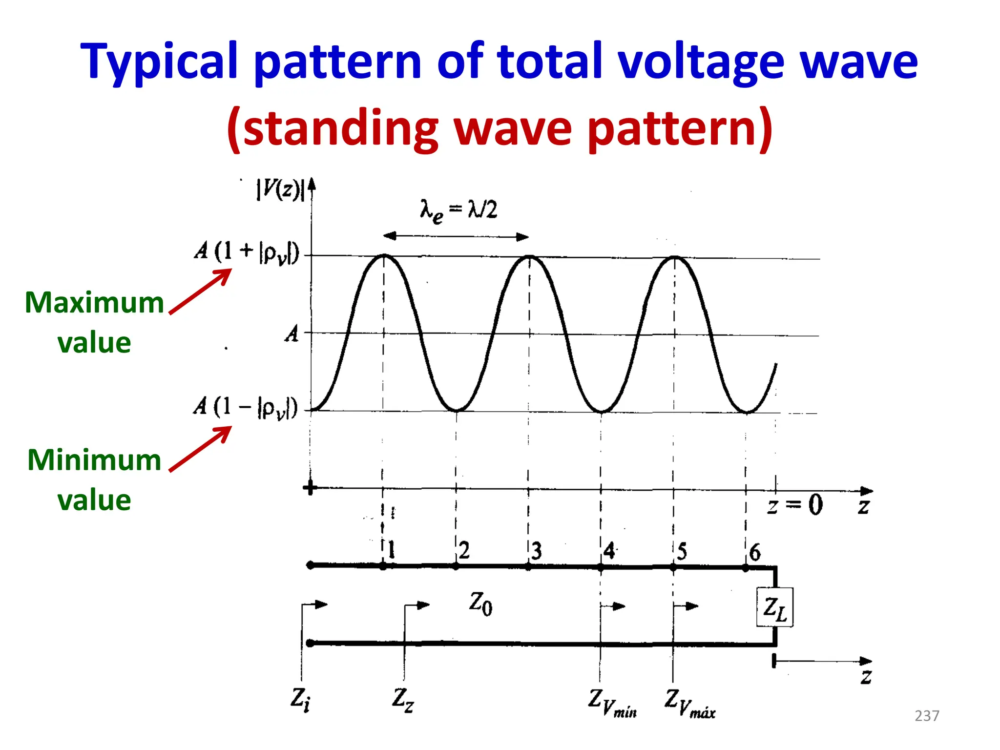
Typical pattern oftotal voltage wave
(standing wave pattern)
Maximum
value
Minimum
value
237
238.
Standing waves
• Thetotal voltage wave pattern is
periodic and is called a standing
wave pattern.
• Incident and reflected wave period
= βz.
• Total wave period (superposition of
the previous two waves) = 2βz.
238
239.
Standing waves
• Ifthe incident wave has a wavelength λ,
the standing wave will have a
wavelength λe = λ/2.
• In the graph, points 1, 3, and 5 are of
maximum voltage, and points 2, 4, and 6
are of minimum voltage in the standing
wave.
239
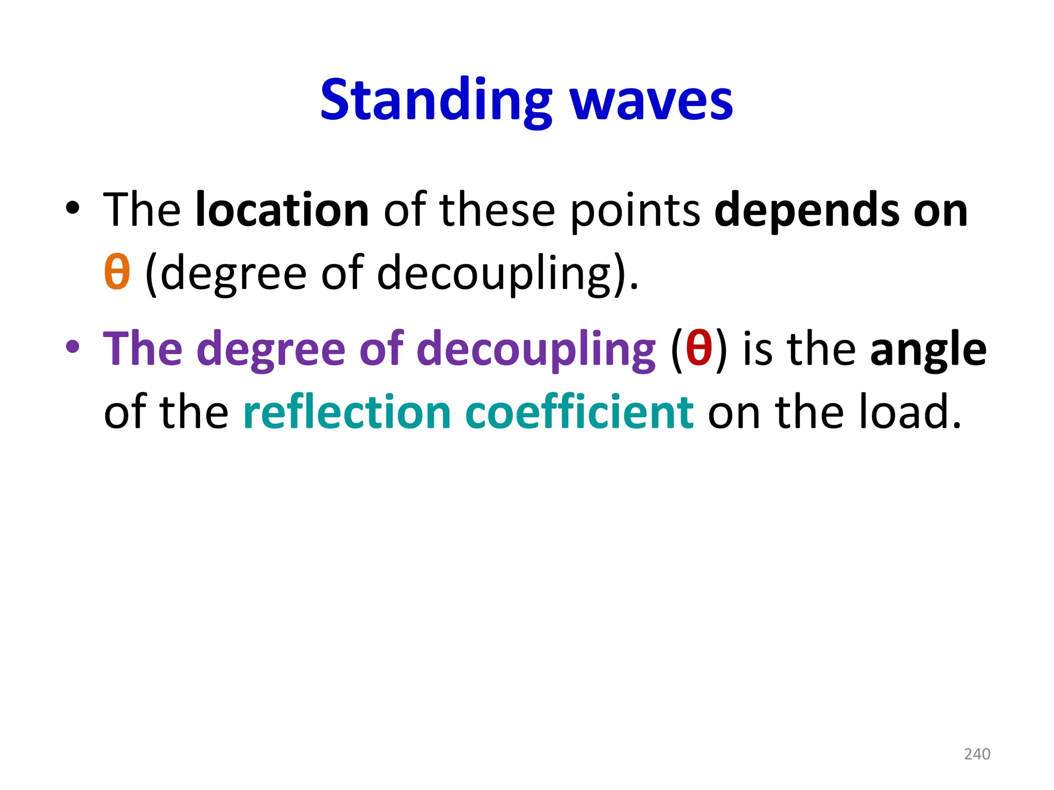
240.
Standing waves
• Thelocation of these points depends on
θ (degree of decoupling).
• The degree of decoupling (θ) is the angle
of the reflection coefficient on the load.
240
241.
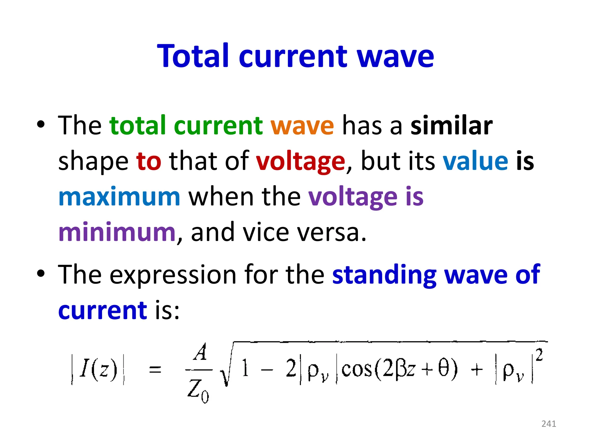
Total current wave
•The total current wave has a similar
shape to that of voltage, but its value is
maximum when the voltage is
minimum, and vice versa.
• The expression for the standing wave of
current is:
241
242.
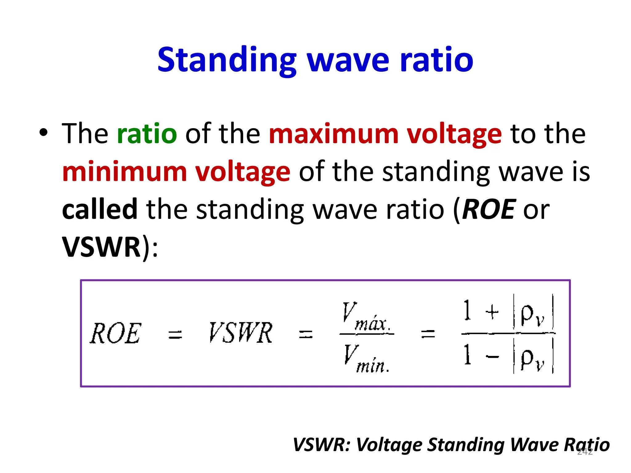
Standing wave ratio
•The ratio of the maximum voltage to the
minimum voltage of the standing wave is
called the standing wave ratio (ROE or
VSWR):
VSWR: Voltage Standing Wave Ratio
242
243.
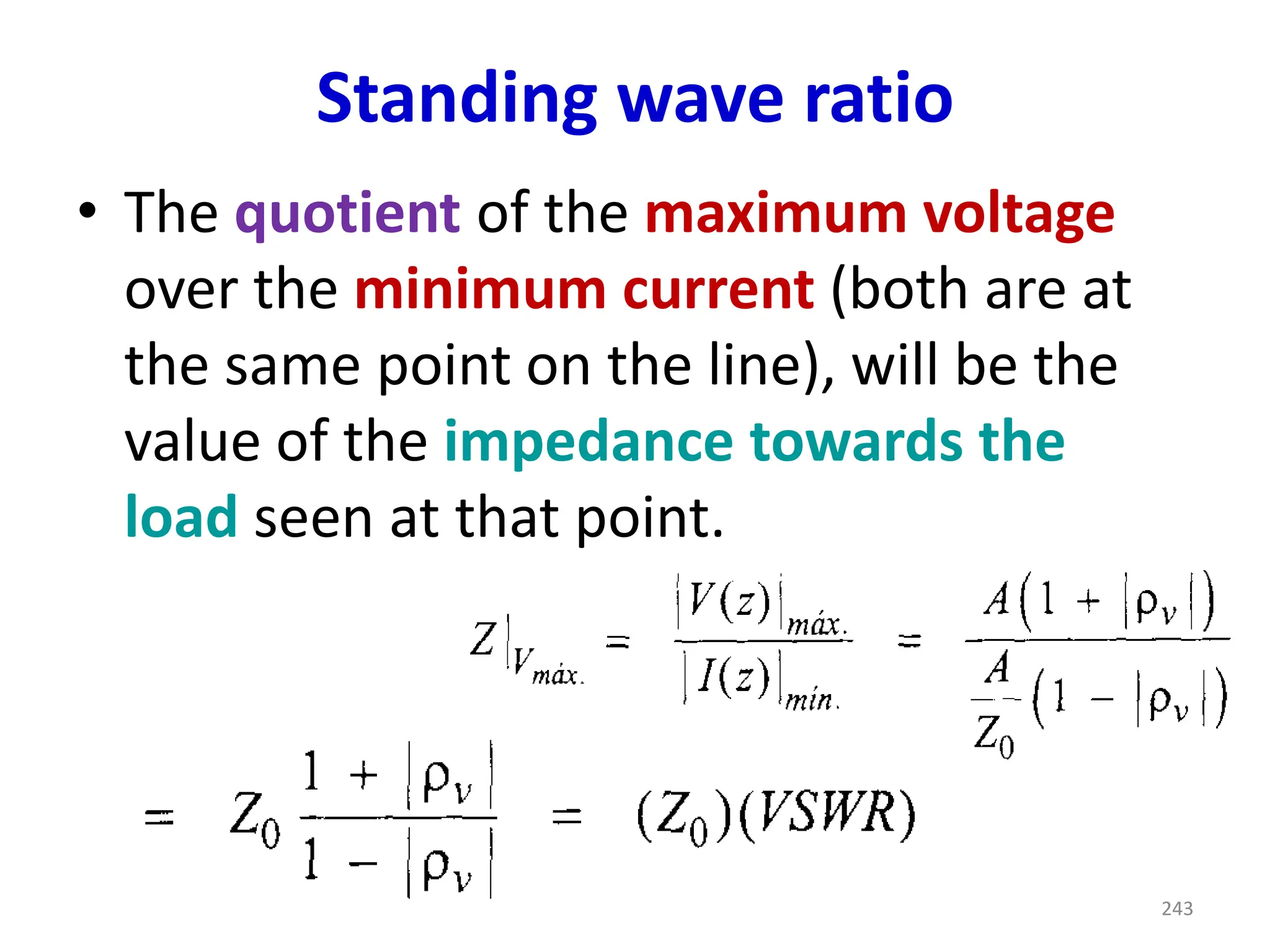
Standing wave ratio
•The quotient of the maximum voltage
over the minimum current (both are at
the same point on the line), will be the
value of the impedance towards the
load seen at that point.
243
244.
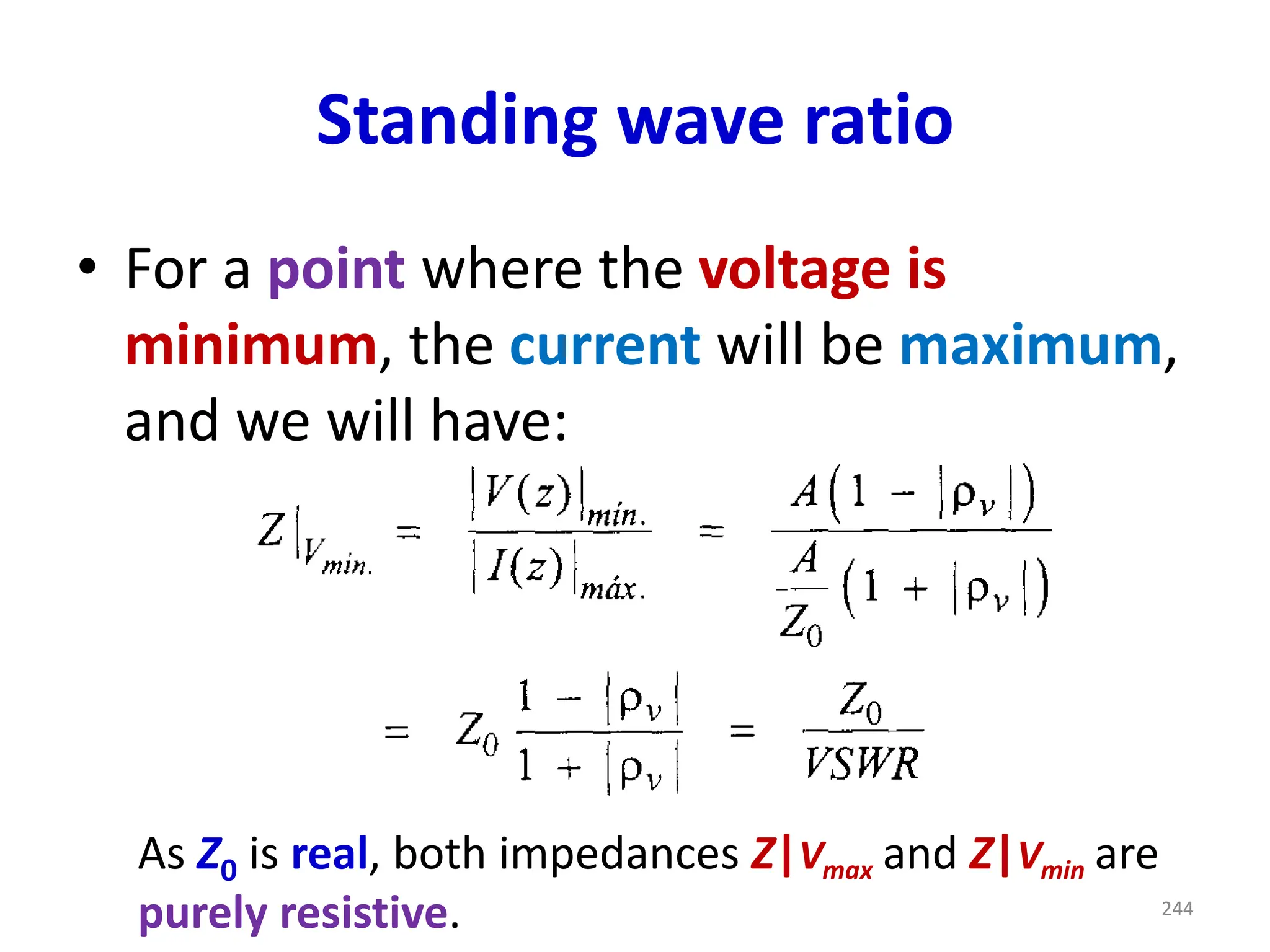
Standing wave ratio
•For a point where the voltage is
minimum, the current will be maximum,
and we will have:
As Z0 is real, both impedances Z|Vmax and Z|Vmin are
purely resistive. 244
245.
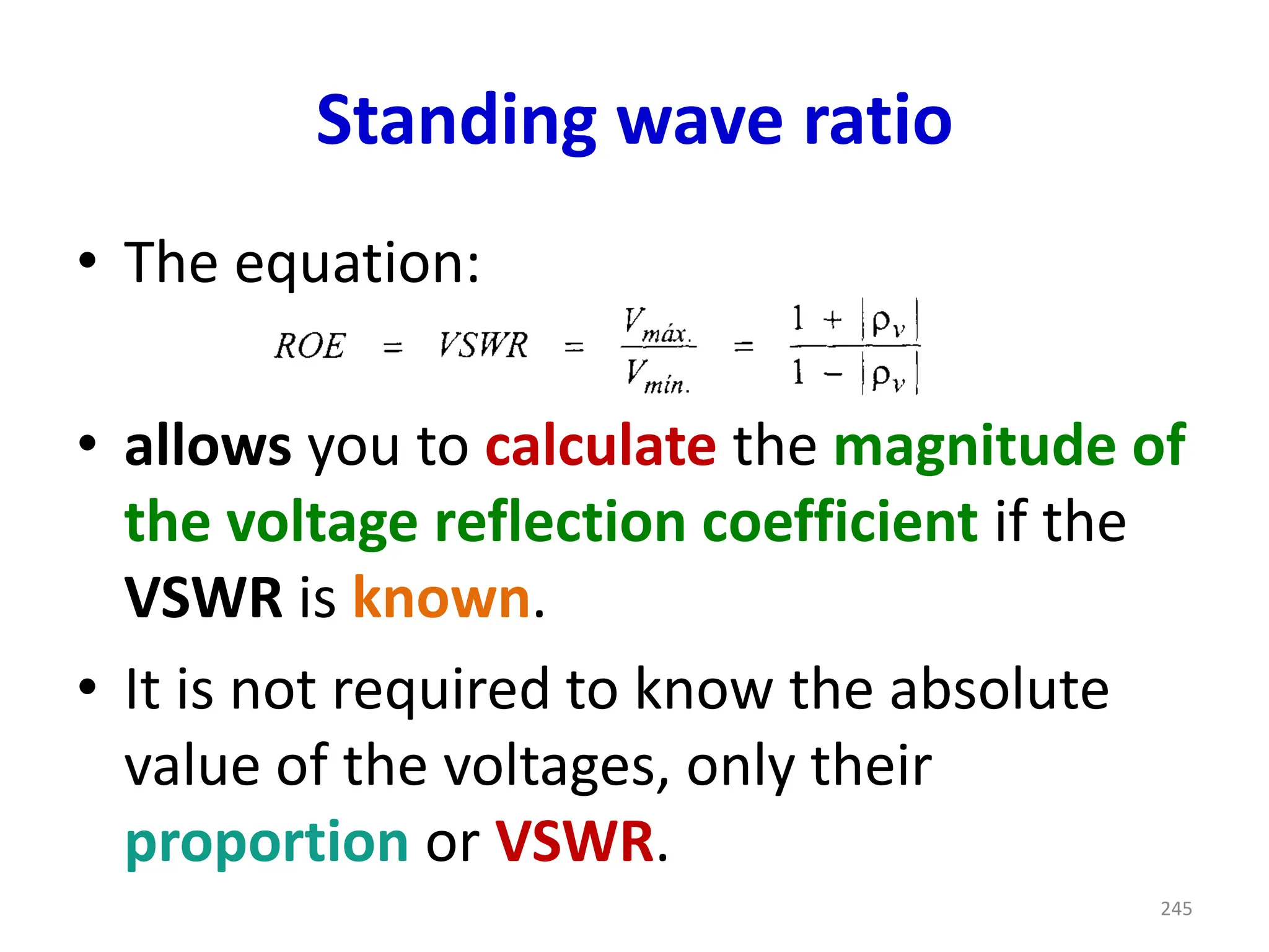
Standing wave ratio
•The equation:
• allows you to calculate the magnitude of
the voltage reflection coefficient if the
VSWR is known.
• It is not required to know the absolute
value of the voltages, only their
proportion or VSWR.
245
246.
Standing wave ratio
•The VSWR can be measured indirectly
in a laboratory with a standing wave
detector.
• It consists of a rigid coaxial line, with a
longitudinal slot at its top, through
which a small electric field (E) probe
slides.
246
247.
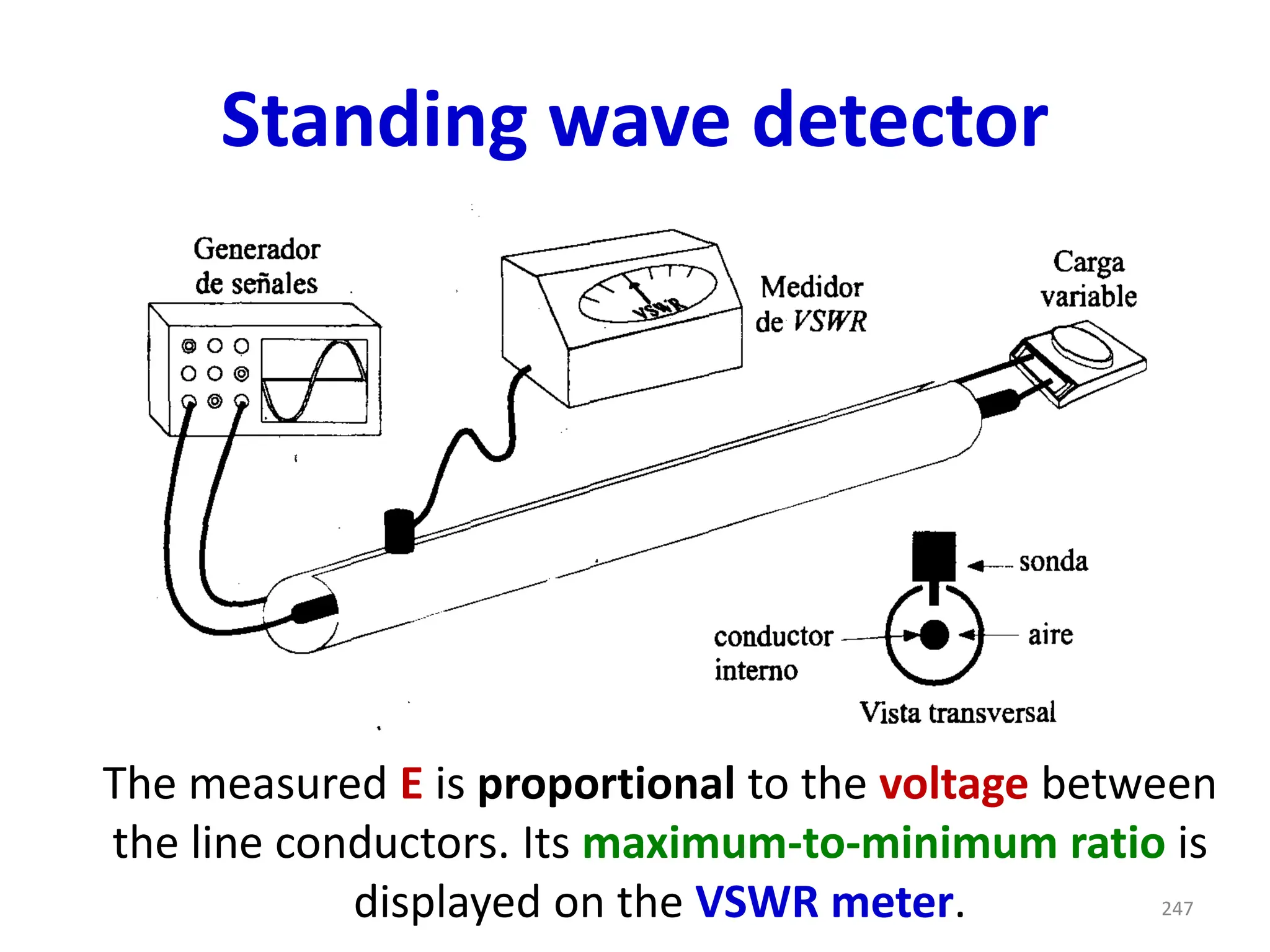
Standing wave detector
Themeasured E is proportional to the voltage between
the line conductors. Its maximum-to-minimum ratio is
displayed on the VSWR meter. 247
248.
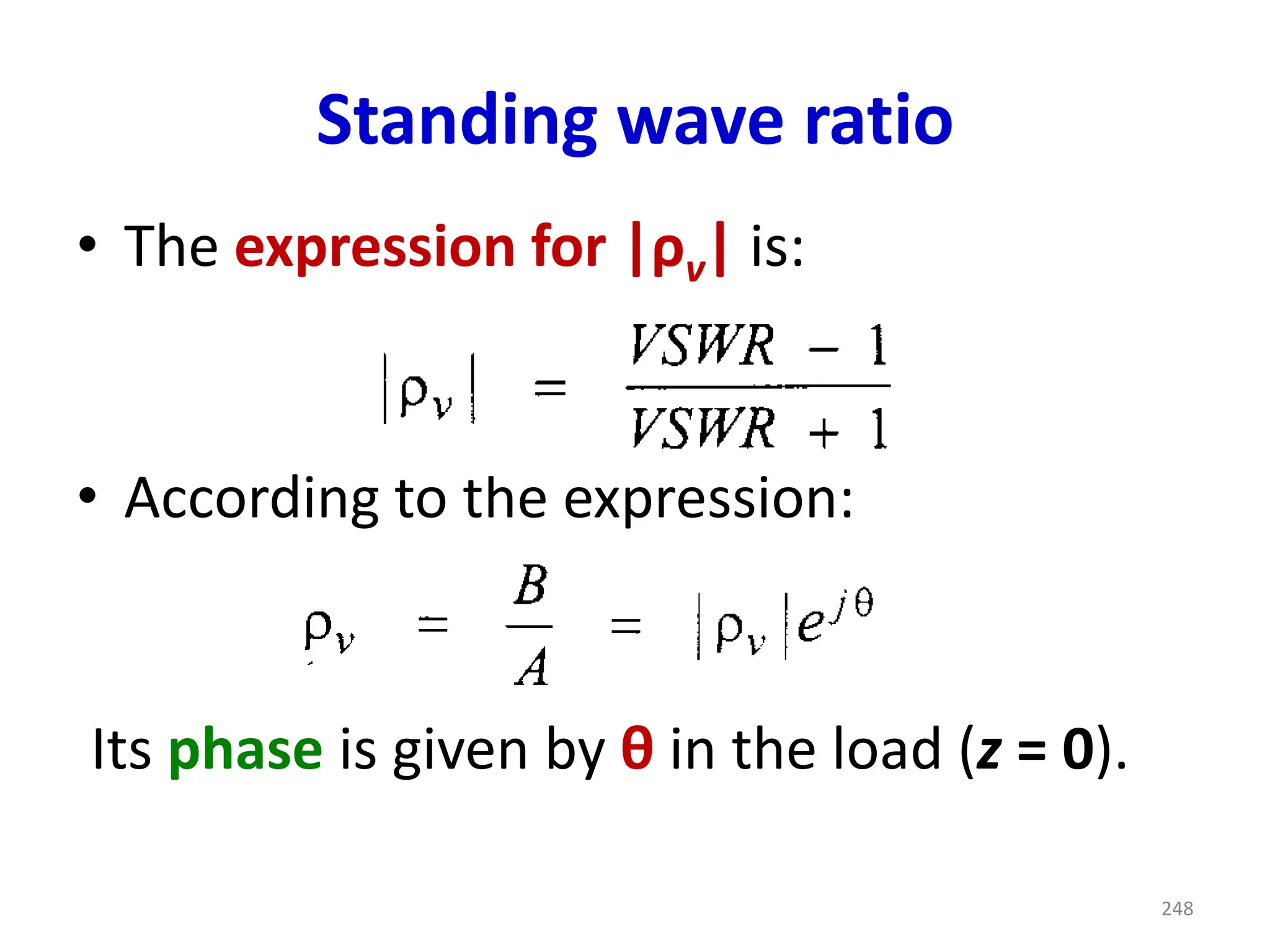
Standing wave ratio
•The expression for |ρv| is:
• According to the expression:
Its phase is given by θ in the load (z = 0).
248
249.
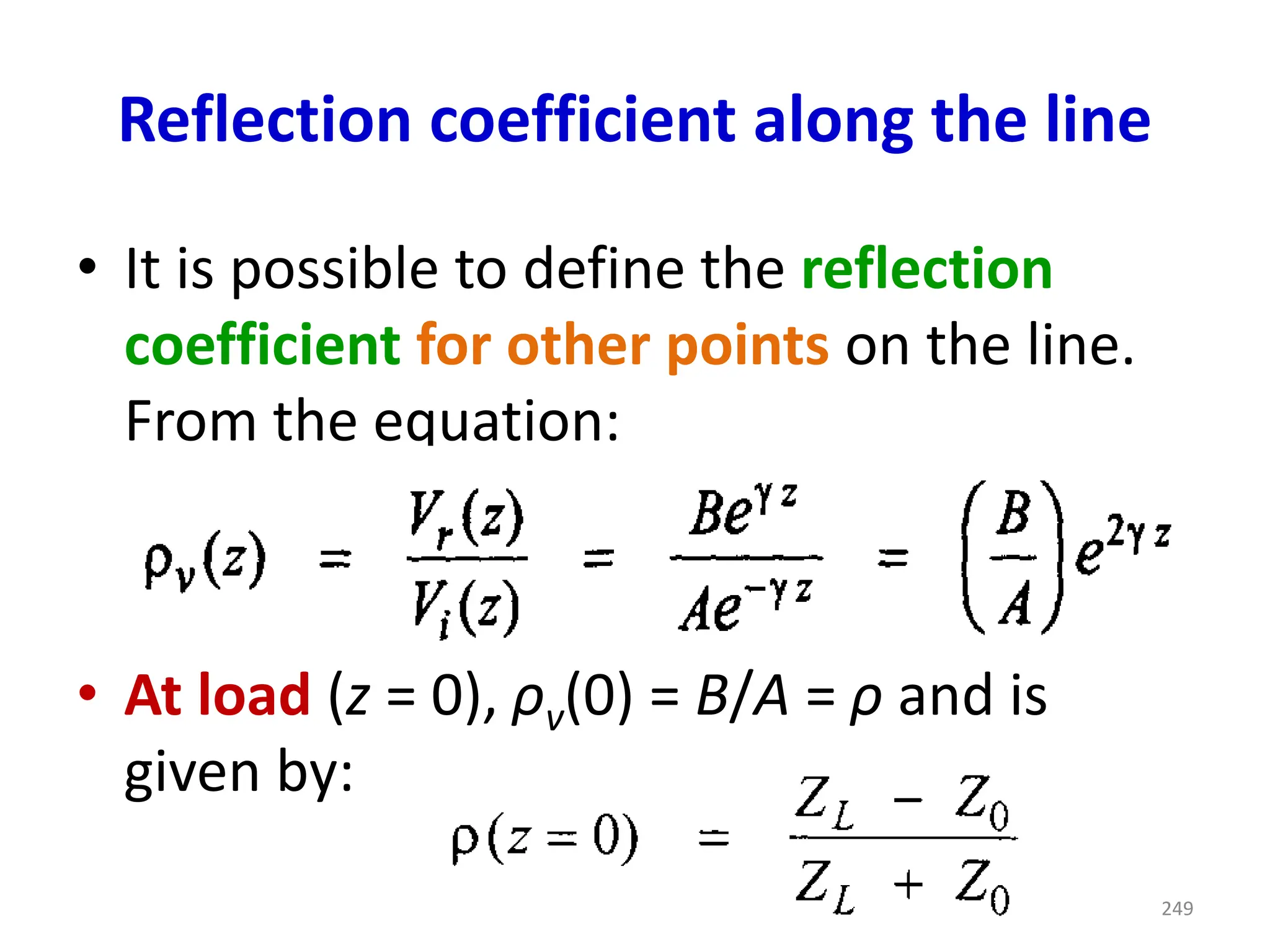
Reflection coefficient alongthe line
• It is possible to define the reflection
coefficient for other points on the line.
From the equation:
• At load (z = 0), ρv(0) = B/A = ρ and is
given by:
249
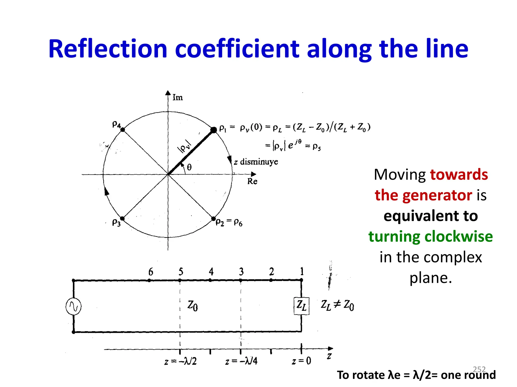
Reflection coefficient alongthe line
• From the above equation it follows
that the geometric place of the
voltage reflection coefficient in the
complex plane is a circle of radius
|ρv|.
• Its value is repeated every time λe =
λ/2 is advanced along the line.
251
252.
Reflection coefficient alongthe line
Moving towards
the generator is
equivalent to
turning clockwise
in the complex
plane.
To rotate λe = λ/2= one round
252
253.
Exercise 2-11
• Acoaxial cable with a characteristic
impedance of 100 Ω and air as the
dielectric inside has a load of 80 + j50 Ω
connected to it .
• Obtain the reflection coefficient where
the load is, and at 25 cm measured from
the load towards the generator.
253
254.
Exercise 2-11
• Alsocalculate the value of the VSWR and
the positions of the first minimum and
the first and second maximum voltages,
from the load to the generator. Indicate
these distances in centimeters.
• Consider that the operating frequency is
300 MHz.
254
255.
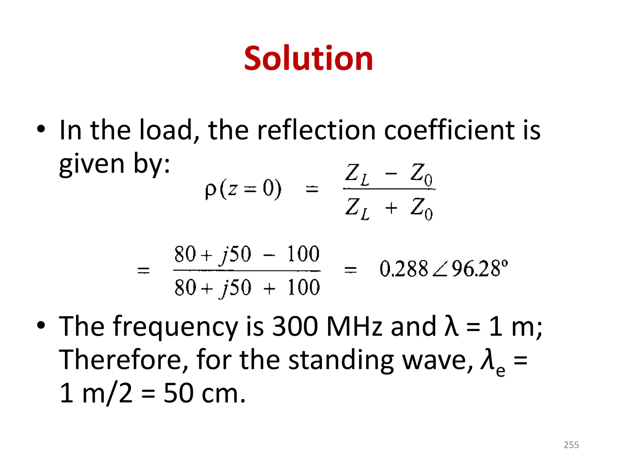
Solution
• In theload, the reflection coefficient is
given by:
• The frequency is 300 MHz and λ = 1 m;
Therefore, for the standing wave, λe =
1 m/2 = 50 cm.
255
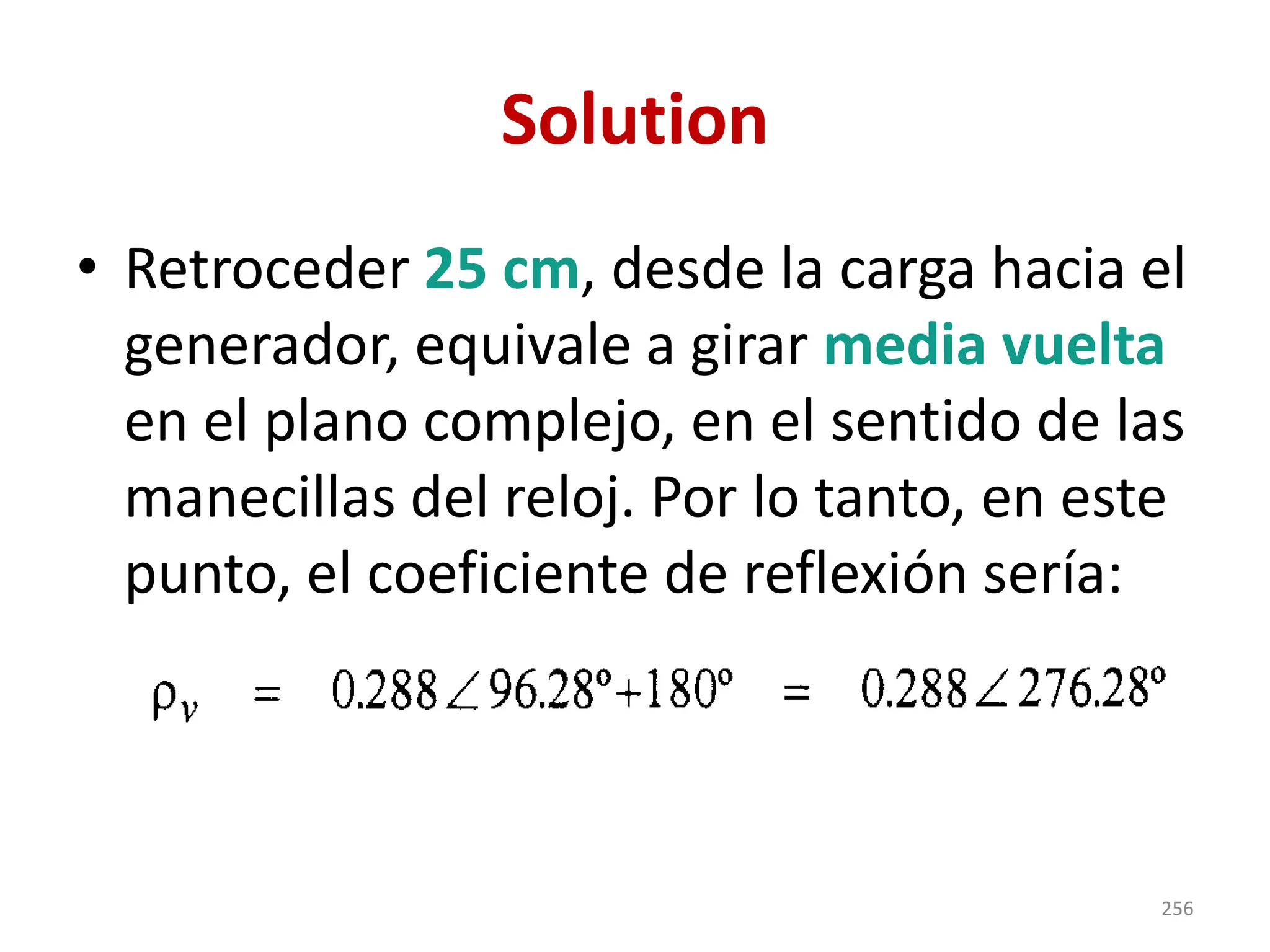
256.
Solution
• Retroceder 25cm, desde la carga hacia el
generador, equivale a girar media vuelta
en el plano complejo, en el sentido de las
manecillas del reloj. Por lo tanto, en este
punto, el coeficiente de reflexión sería:
256
257.
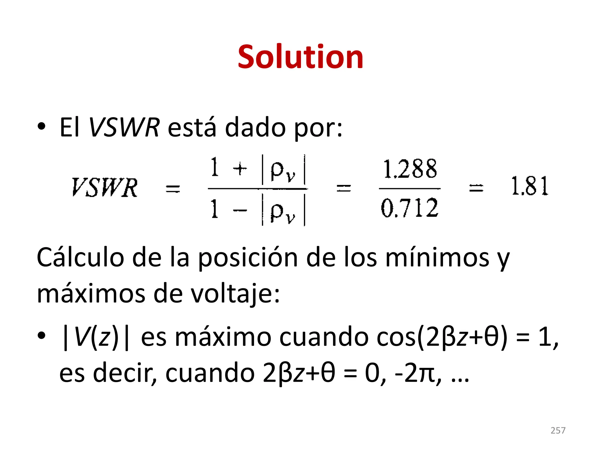
Solution
• El VSWRestá dado por:
Cálculo de la posición de los mínimos y
máximos de voltaje:
• |V(z)| es máximo cuando cos(2βz+θ) = 1,
es decir, cuando 2βz+θ = 0, -2π, …
257
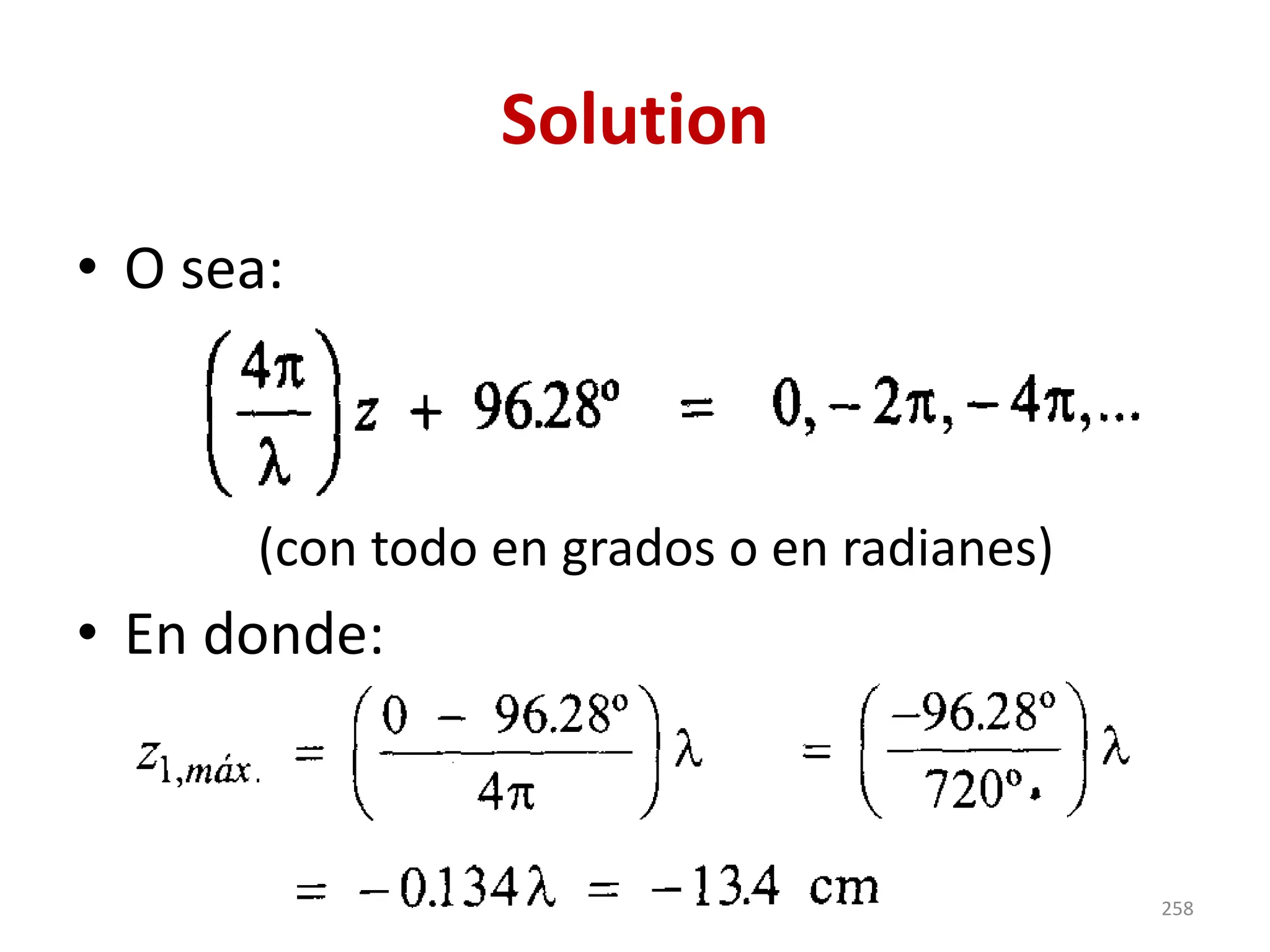
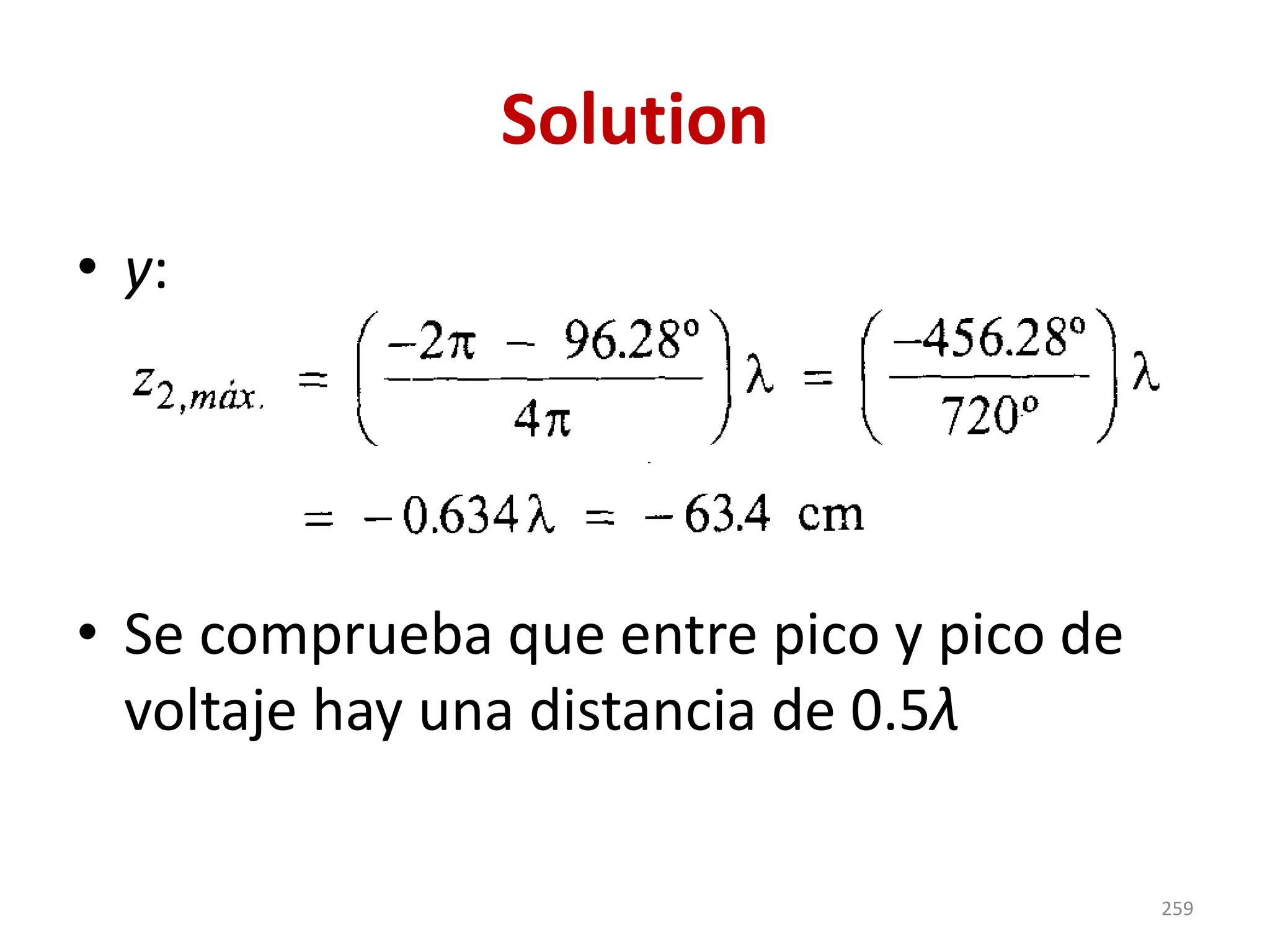
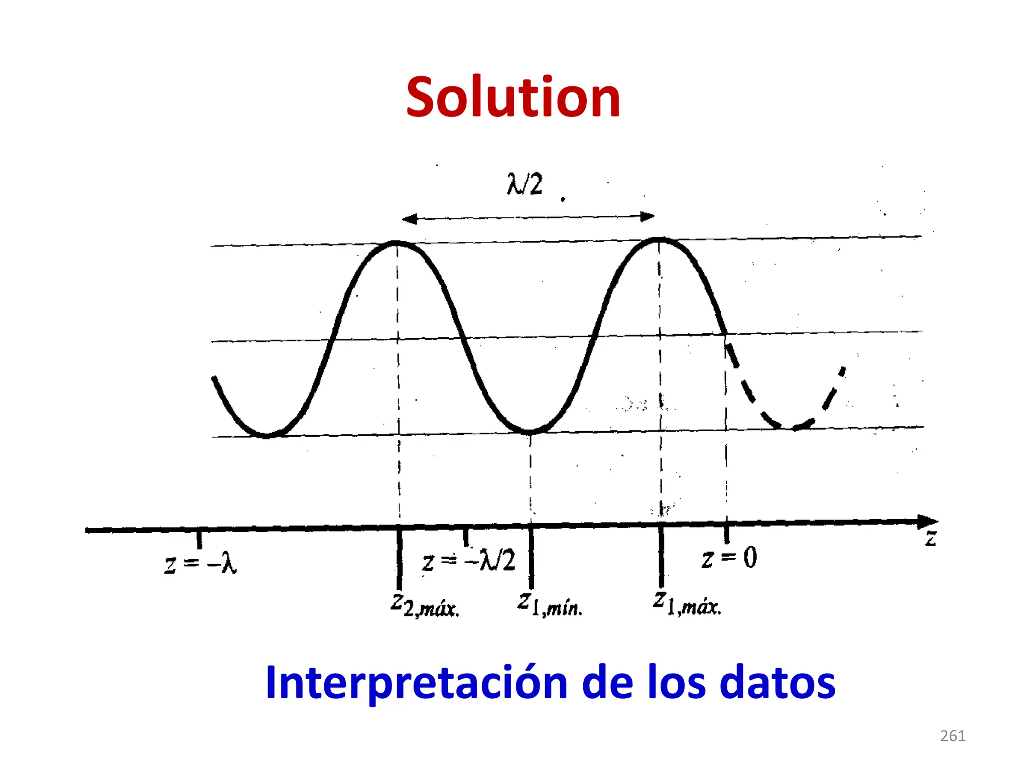
Solution
• y:
• Secomprueba que entre pico y pico de
voltaje hay una distancia de 0.5λ
259
260.
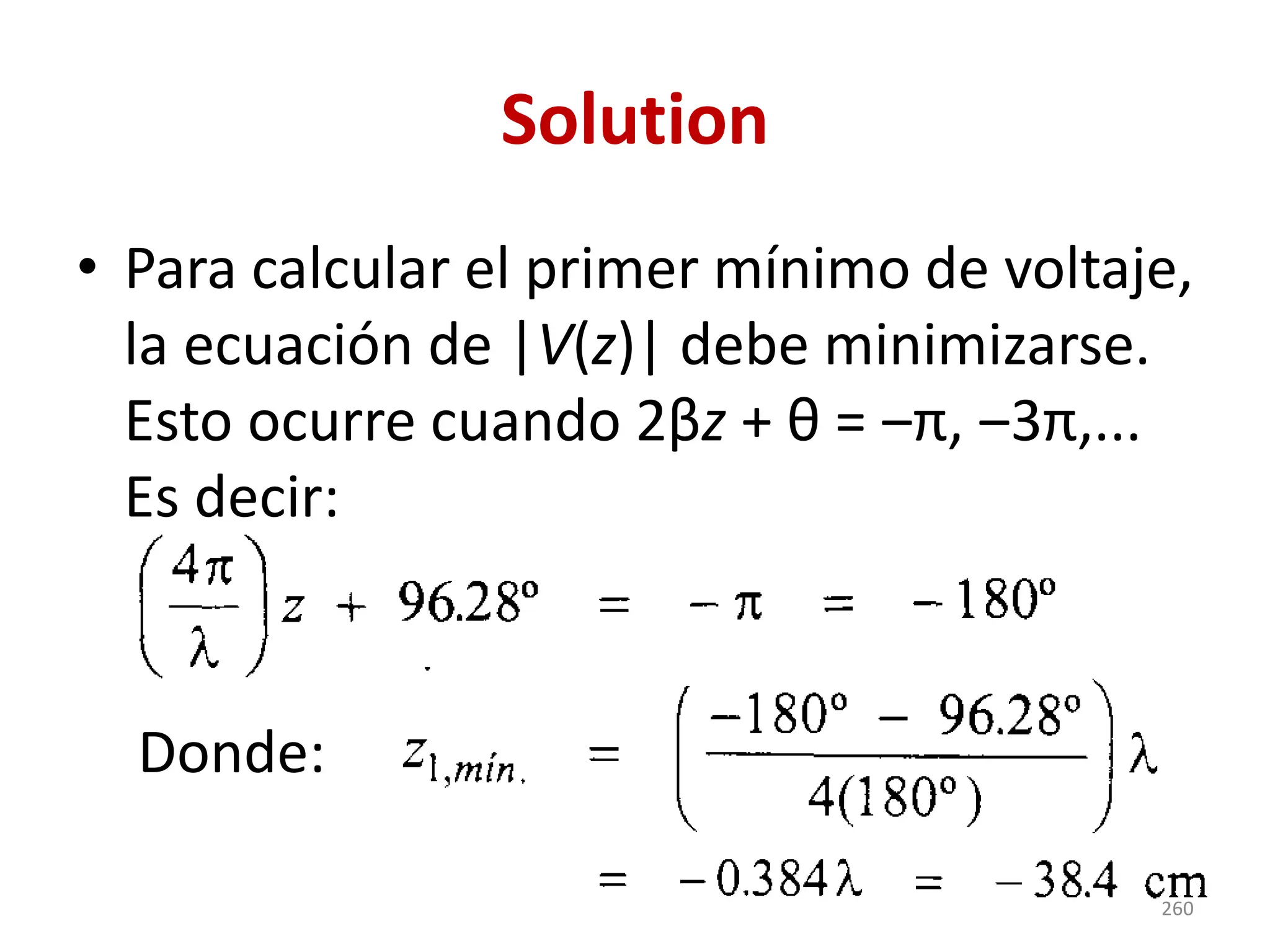
Solution
• Para calcularel primer mínimo de voltaje,
la ecuación de |V(z)| debe minimizarse.
Esto ocurre cuando 2βz + θ = ‒π, ‒3π,...
Es decir:
Donde:
260
Exercise 2-12
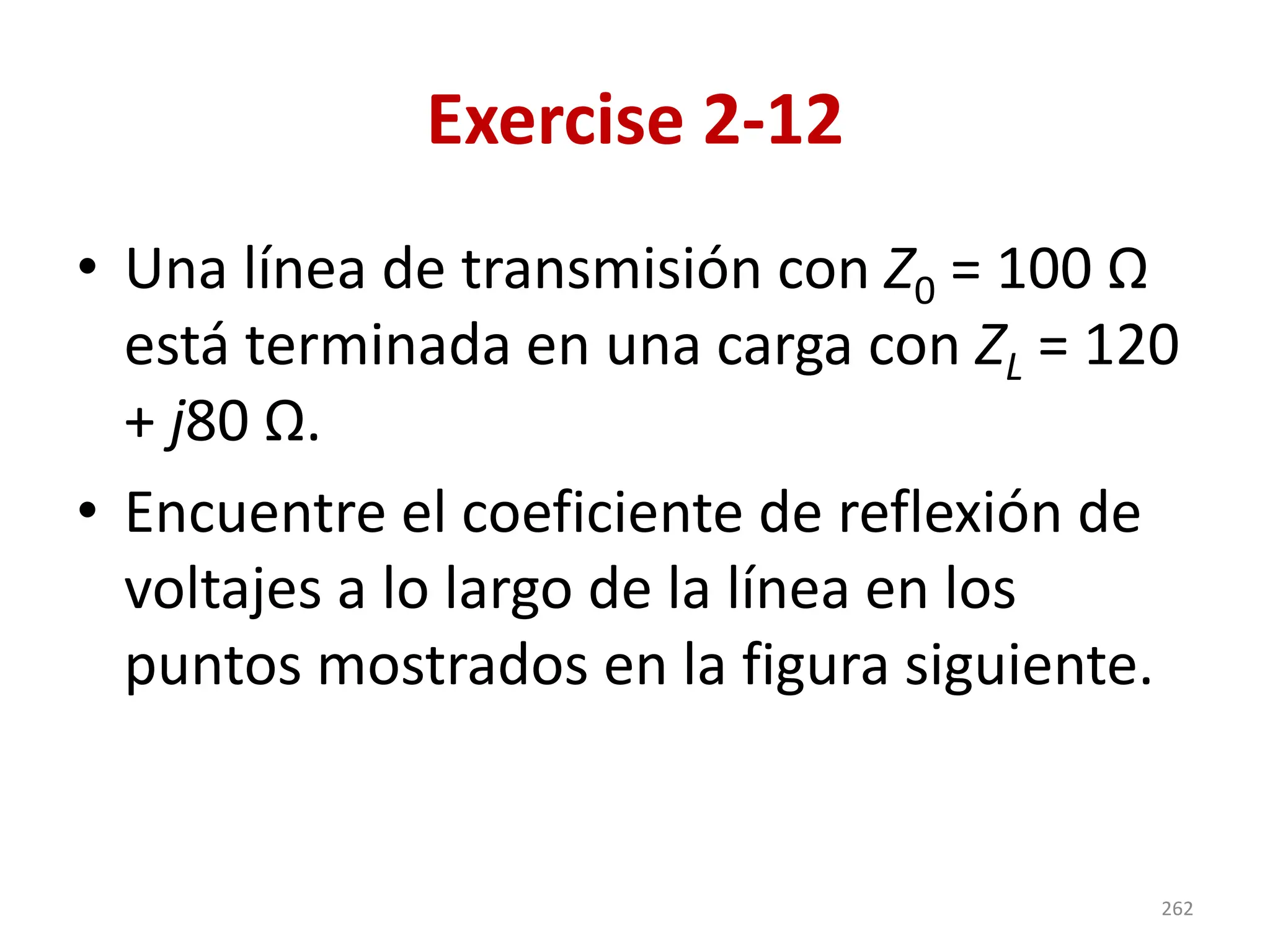
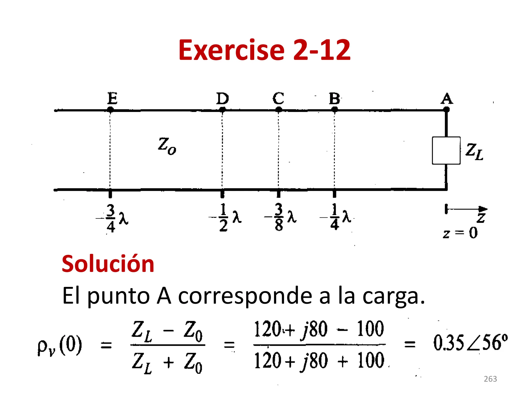
• Unalínea de transmisión con Z0 = 100 Ω
está terminada en una carga con ZL = 120
+ j80 Ω.
• Encuentre el coeficiente de reflexión de
voltajes a lo largo de la línea en los
puntos mostrados en la figura siguiente.
262
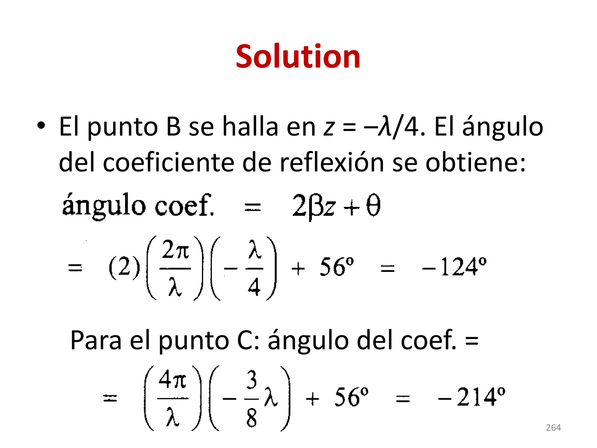
Solution
• El puntoB se halla en z = ‒λ/4. El ángulo
del coeficiente de reflexión se obtiene:
Para el punto C: ángulo del coef. =
264
265.
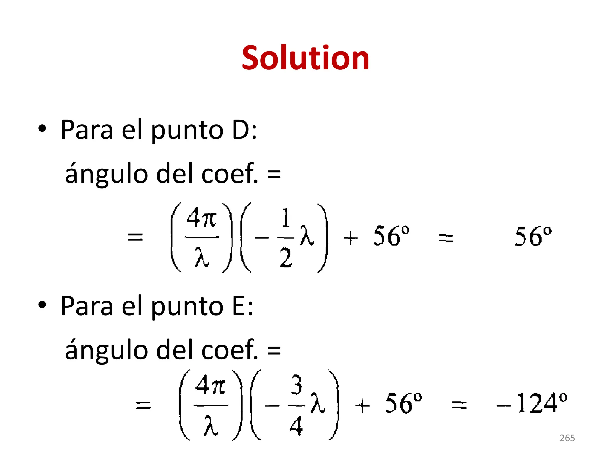
Solution
• Para elpunto D:
ángulo del coef. =
• Para el punto E:
ángulo del coef. =
265
266.
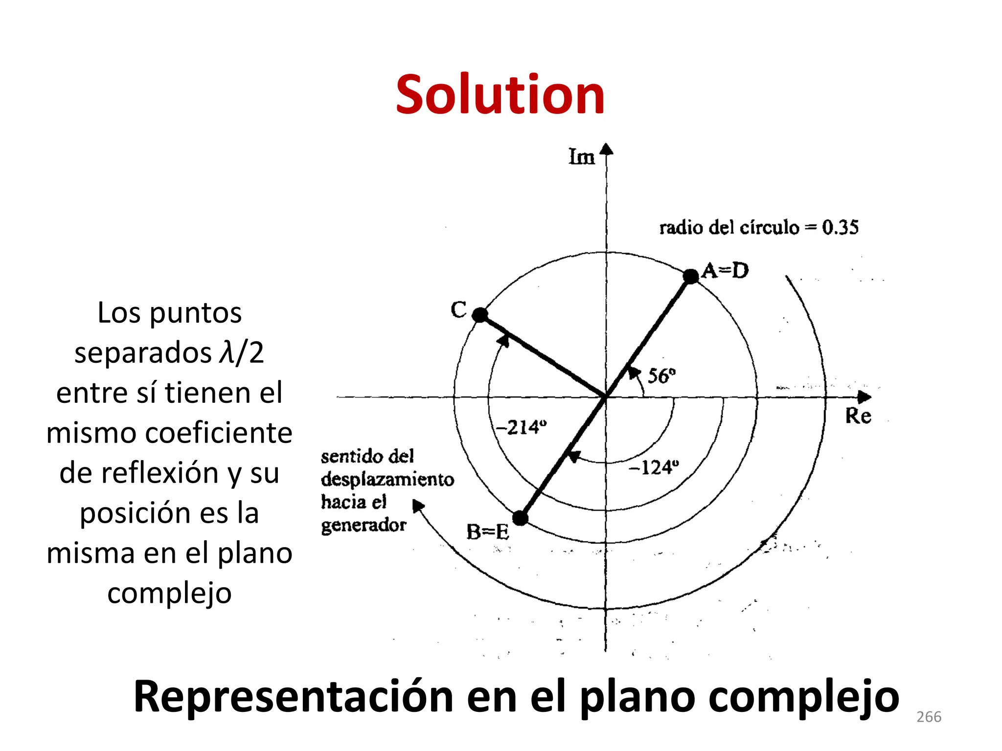
Solution
Representación en elplano complejo
Los puntos
separados λ/2
entre sí tienen el
mismo coeficiente
de reflexión y su
posición es la
misma en el plano
complejo
266
267.
Exercise 2-13
• Determineel valor del VSWR que tendría
una línea cualquiera, sin pérdidas,
cuando al final se tuviese: a) una carga
con impedancia igual a la característica,
b) un corto circuito, y c) un circuito
abierto.
267
268.
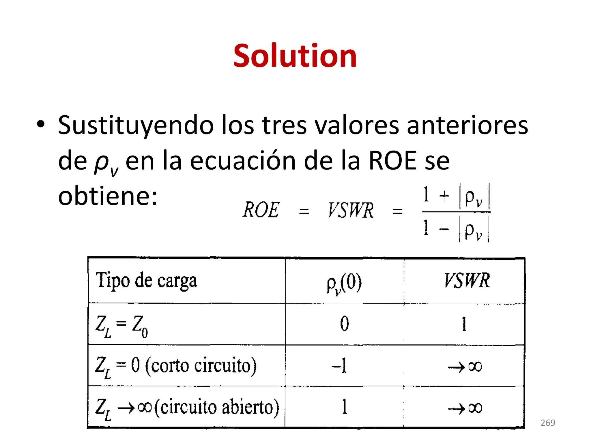
Solution
• Cuando ZL= Z0, la línea está acoplada y
no se refleja nada. Por lo tanto, ρv = 0.
• Cuando la línea termina en un corto
circuito, el voltaje total en ese punto vale
cero. Por lo tanto, ρv = ‒1.
• Cuando la línea termina en circuito
abierto, el voltaje total en ese punto es
máximo. Por lo tanto, ρv = +1.
268
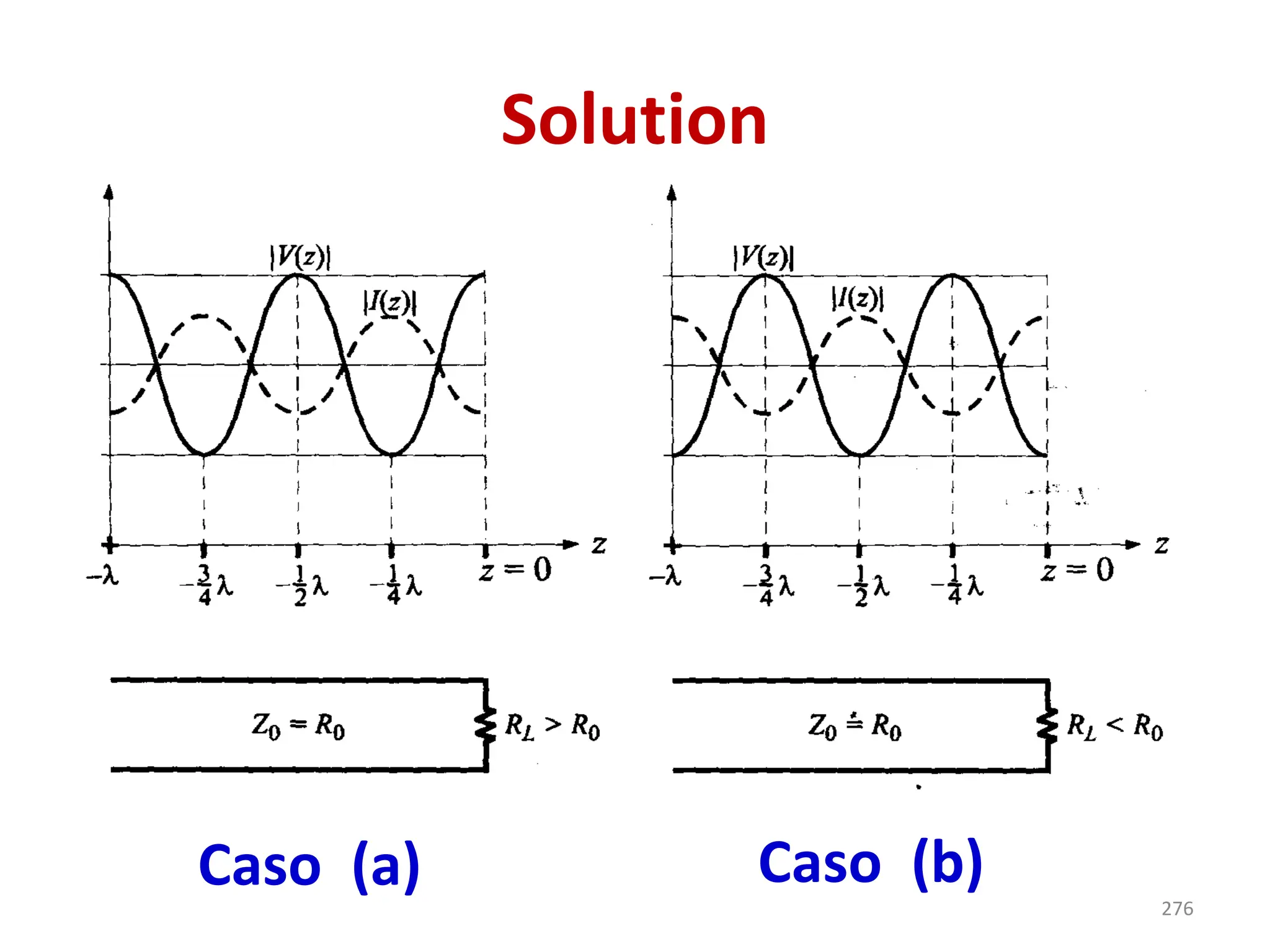
Exercise 2-14
• Grafiquela forma de las ondas
estacionarias de voltaje y corriente para
una línea cualquiera sin pérdidas, cuando
ésta termina en: a) una resistencia pura
mayor que Z0, b) una resistencia pura
menor que Z0, c) un corto circuito, y d) un
circuito abierto.
270
271.
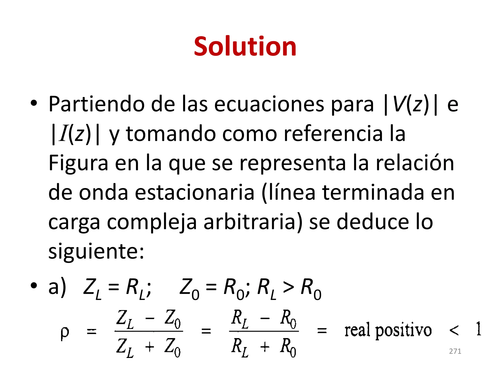
Solution
• Partiendo delas ecuaciones para |V(z)| e
|I(z)| y tomando como referencia la
Figura en la que se representa la relación
de onda estacionaria (línea terminada en
carga compleja arbitraria) se deduce lo
siguiente:
• a) ZL = RL; Z0 = R0; RL > R0
271
272.
Solution
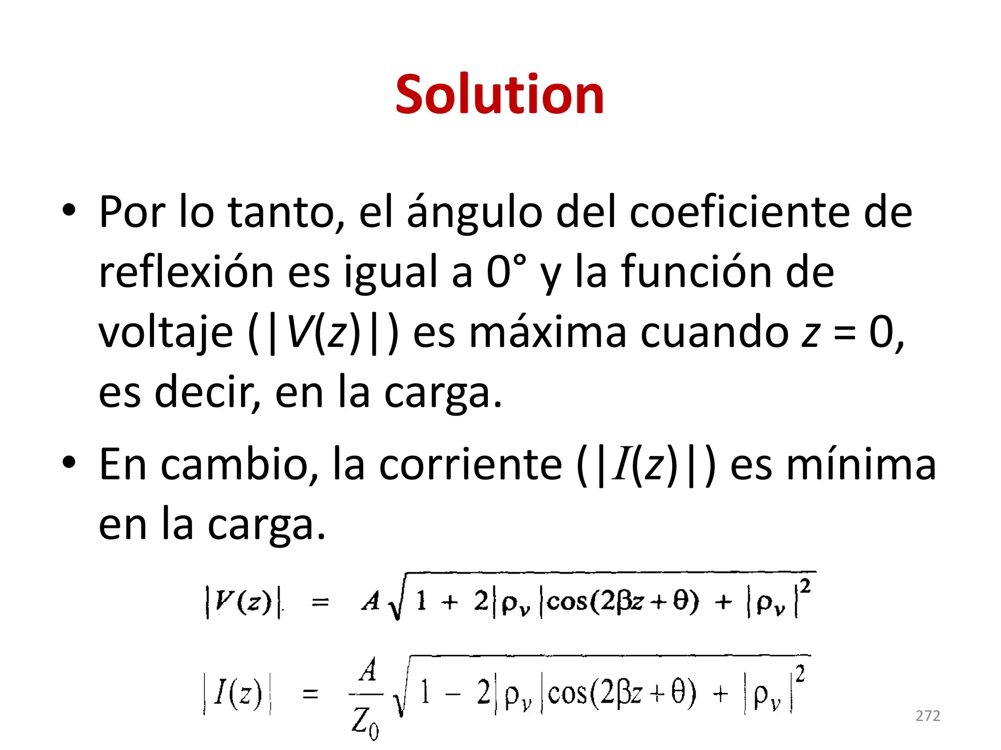
• Por lotanto, el ángulo del coeficiente de
reflexión es igual a 0° y la función de
voltaje (|V(z)|) es máxima cuando z = 0,
es decir, en la carga.
• En cambio, la corriente (|I(z)|) es mínima
en la carga.
272
273.
Solution
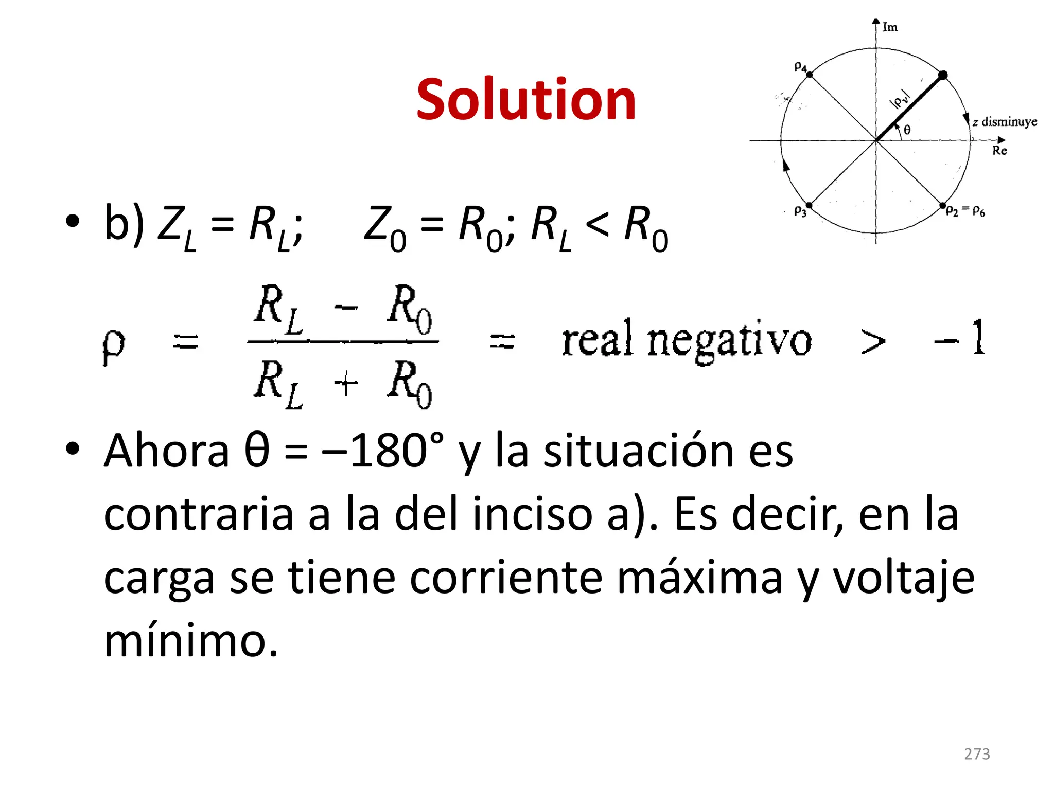
• b) ZL= RL; Z0 = R0; RL < R0
• Ahora θ = ‒180° y la situación es
contraria a la del inciso a). Es decir, en la
carga se tiene corriente máxima y voltaje
mínimo.
273
274.
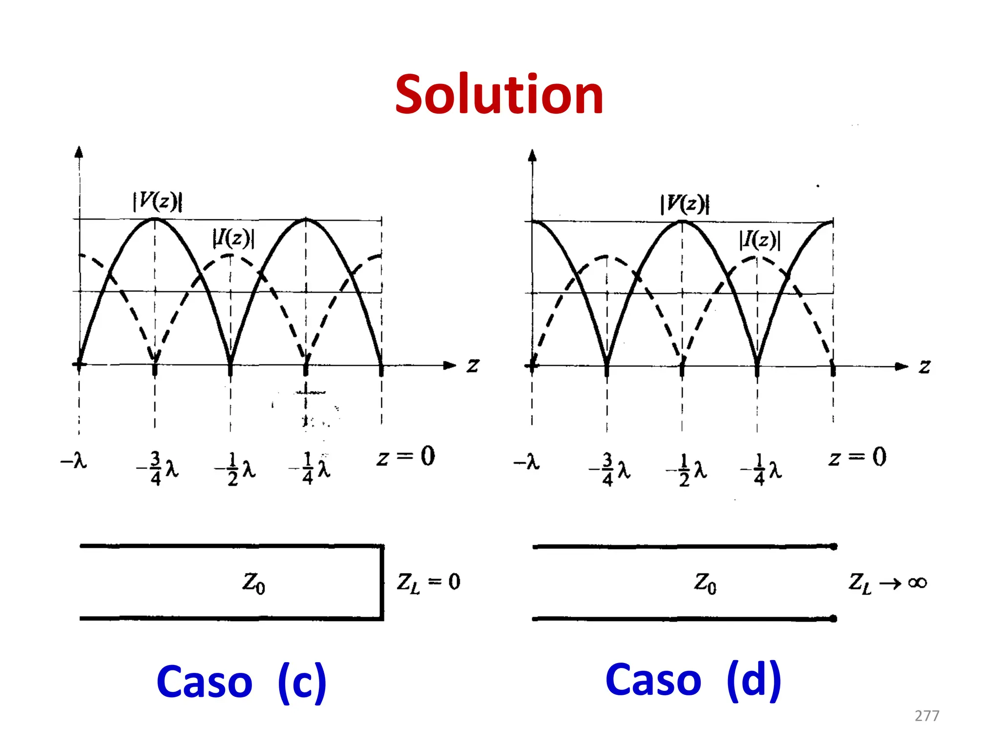
Solution
• c) ZL= 0 (corto circuito)
• Aquí ρ = ‒1 = 1/180° y la situación es
similar a la del inciso b), con corriente
máxima y voltaje mínimo en la carga.
Este voltaje mínimo en la carga ahora
vale cero.
274
275.
Solution
• d) ZL→ ∞ (circuito abierto)
• Como ρ = 1 = 1 / 0° = real positivo, se
tiene algo parecido al inciso a), con
voltaje máximo y corriente mínima en la
carga.
• Esta corriente mínima vale cero.
275
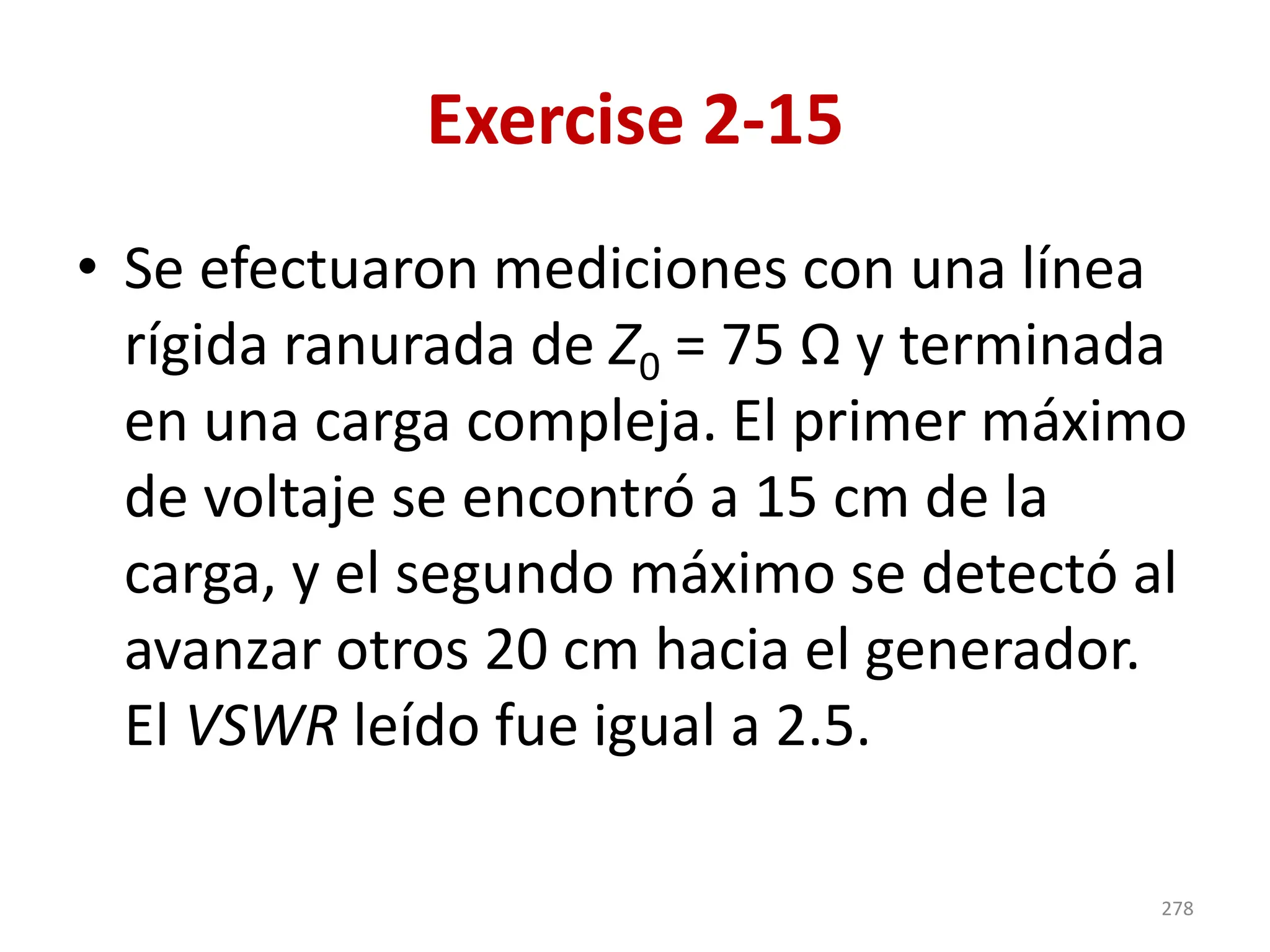
Exercise 2-15
• Seefectuaron mediciones con una línea
rígida ranurada de Z0 = 75 Ω y terminada
en una carga compleja. El primer máximo
de voltaje se encontró a 15 cm de la
carga, y el segundo máximo se detectó al
avanzar otros 20 cm hacia el generador.
El VSWR leído fue igual a 2.5.
278
279.
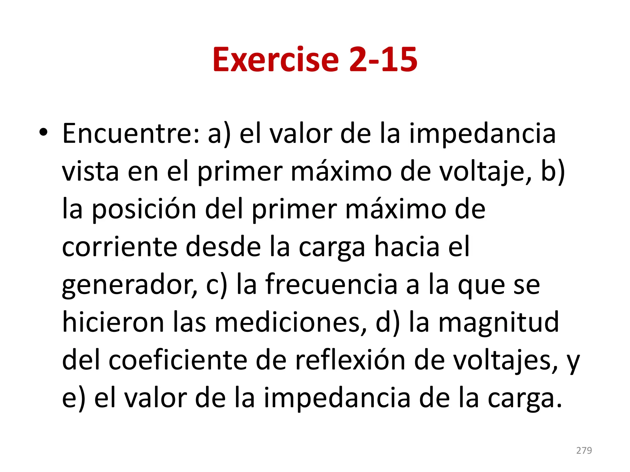
Exercise 2-15
• Encuentre:a) el valor de la impedancia
vista en el primer máximo de voltaje, b)
la posición del primer máximo de
corriente desde la carga hacia el
generador, c) la frecuencia a la que se
hicieron las mediciones, d) la magnitud
del coeficiente de reflexión de voltajes, y
e) el valor de la impedancia de la carga.
279
280.
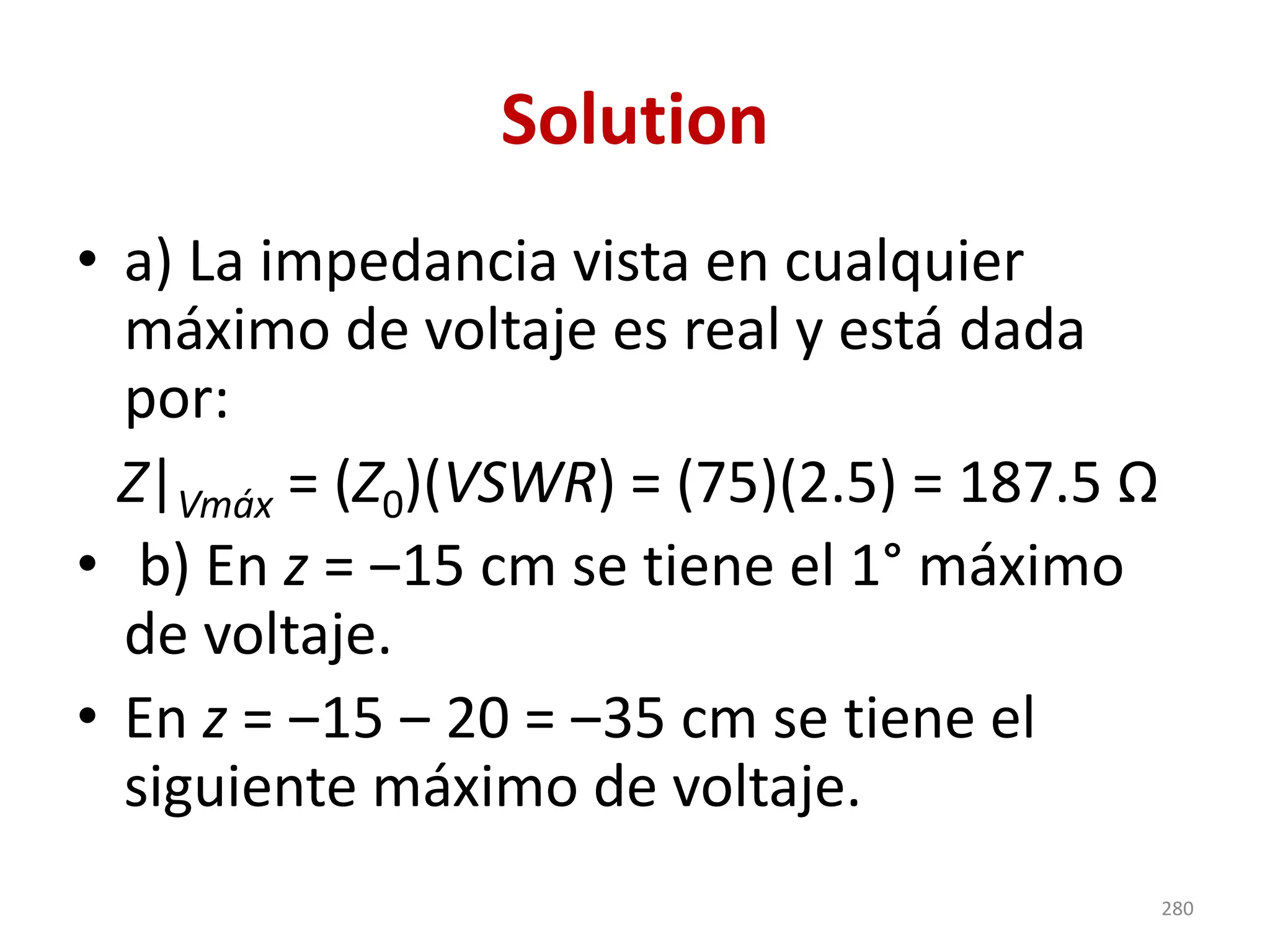
Solution
• a) Laimpedancia vista en cualquier
máximo de voltaje es real y está dada
por:
• b) En z = ‒15 cm se tiene el 1° máximo
de voltaje.
• En z = ‒15 ‒ 20 = ‒35 cm se tiene el
siguiente máximo de voltaje.
Z|Vmáx = (Z0)(VSWR) = (75)(2.5) = 187.5 Ω
280
281.
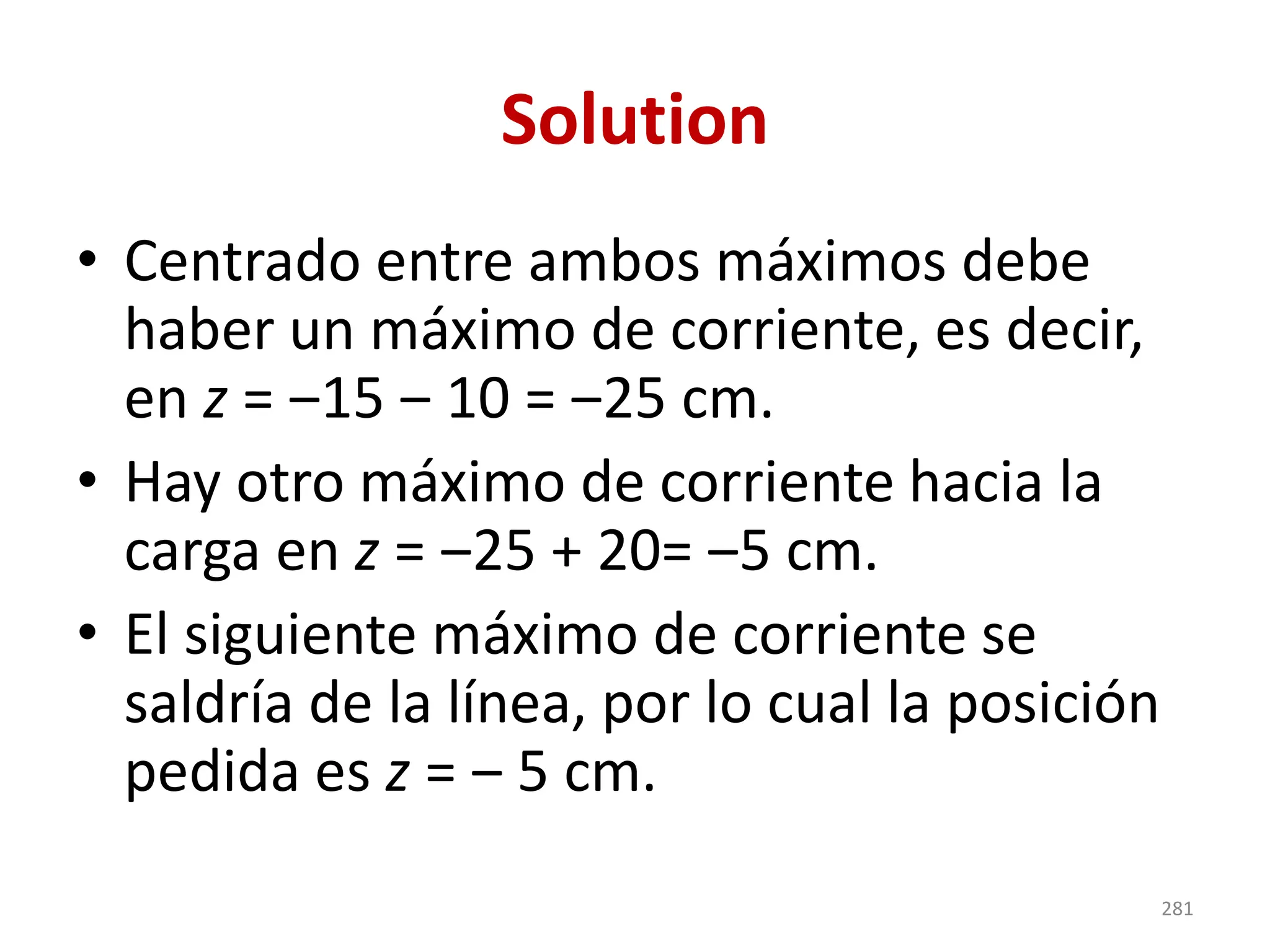
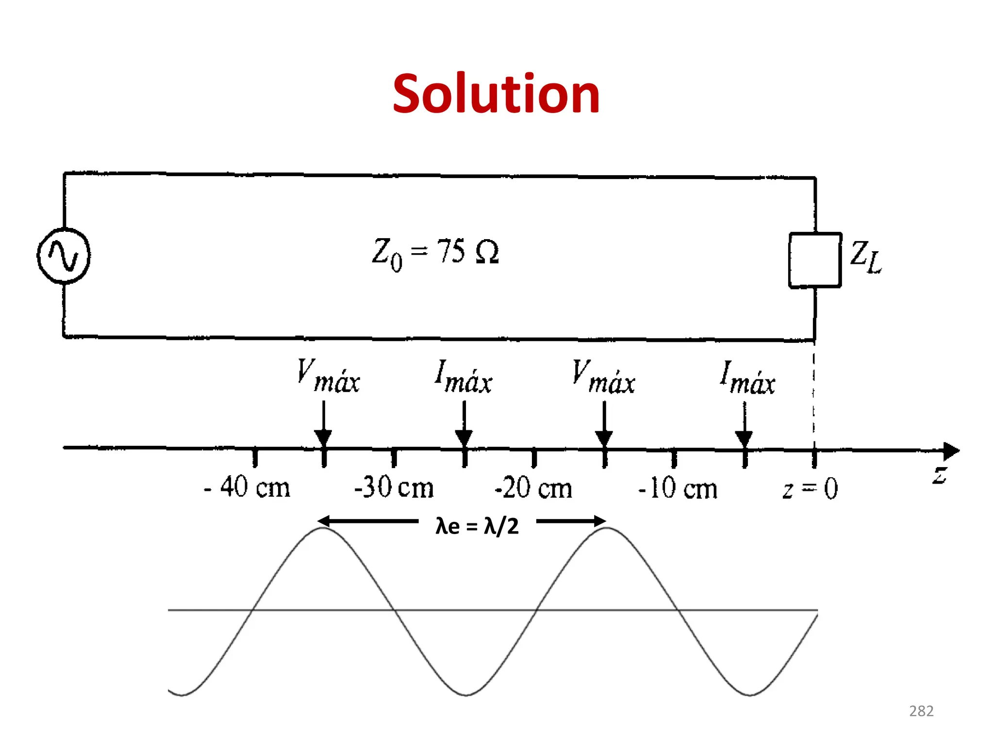
Solution
• Centrado entreambos máximos debe
haber un máximo de corriente, es decir,
en z = ‒15 ‒ 10 = ‒25 cm.
• Hay otro máximo de corriente hacia la
carga en z = ‒25 + 20= ‒5 cm.
• El siguiente máximo de corriente se
saldría de la línea, por lo cual la posición
pedida es z = ‒ 5 cm.
281
Solution
• c) Laλ a la frecuencia de trabajo es el
doble de la distancia entre dos máximos
de voltaje o de corriente de la onda
estacionaria.
λ = (2)(20 cm) = 40 cm.
283
284.
Solution
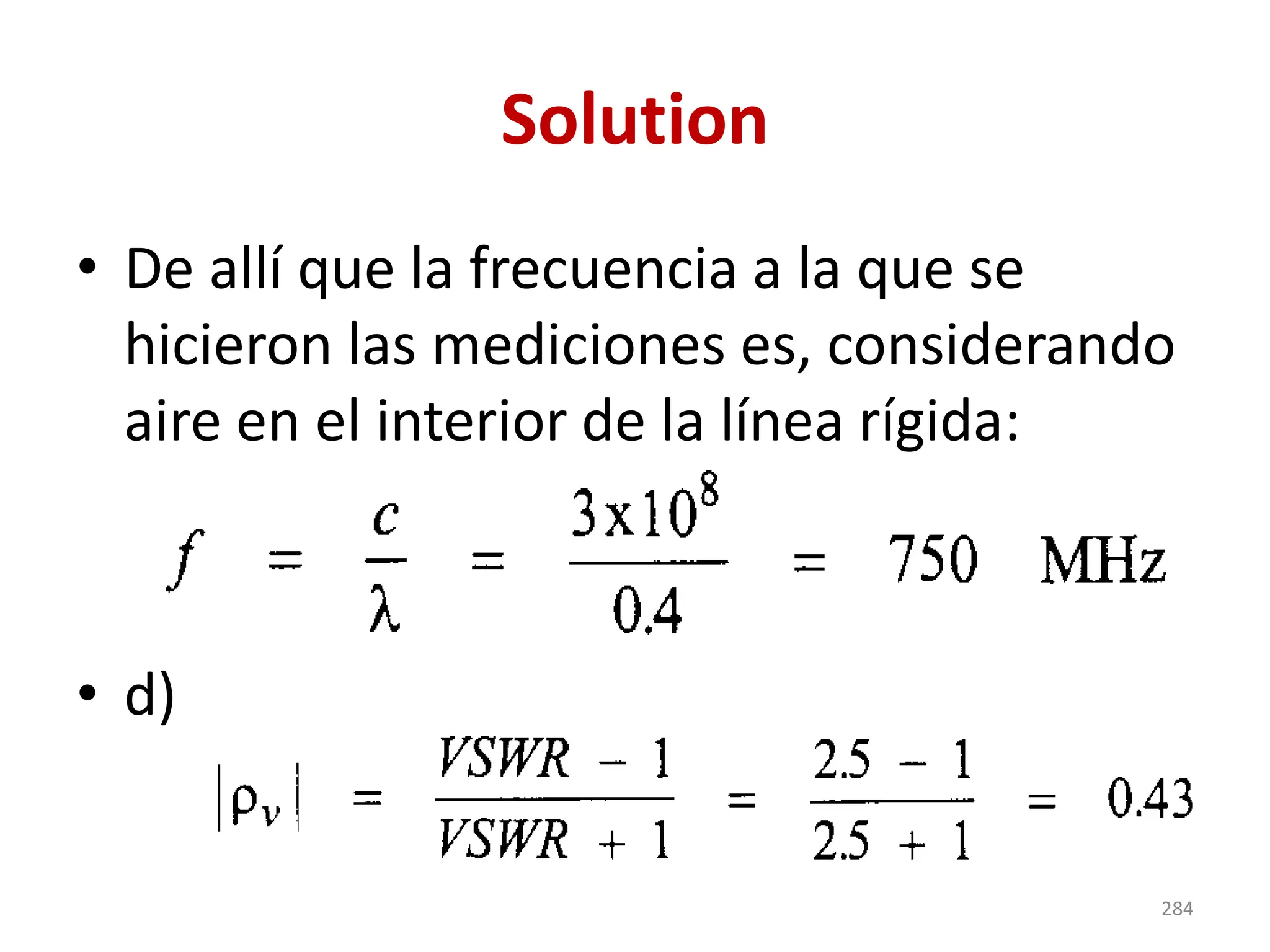
• De allíque la frecuencia a la que se
hicieron las mediciones es, considerando
aire en el interior de la línea rígida:
• d)
284
285.
Solution
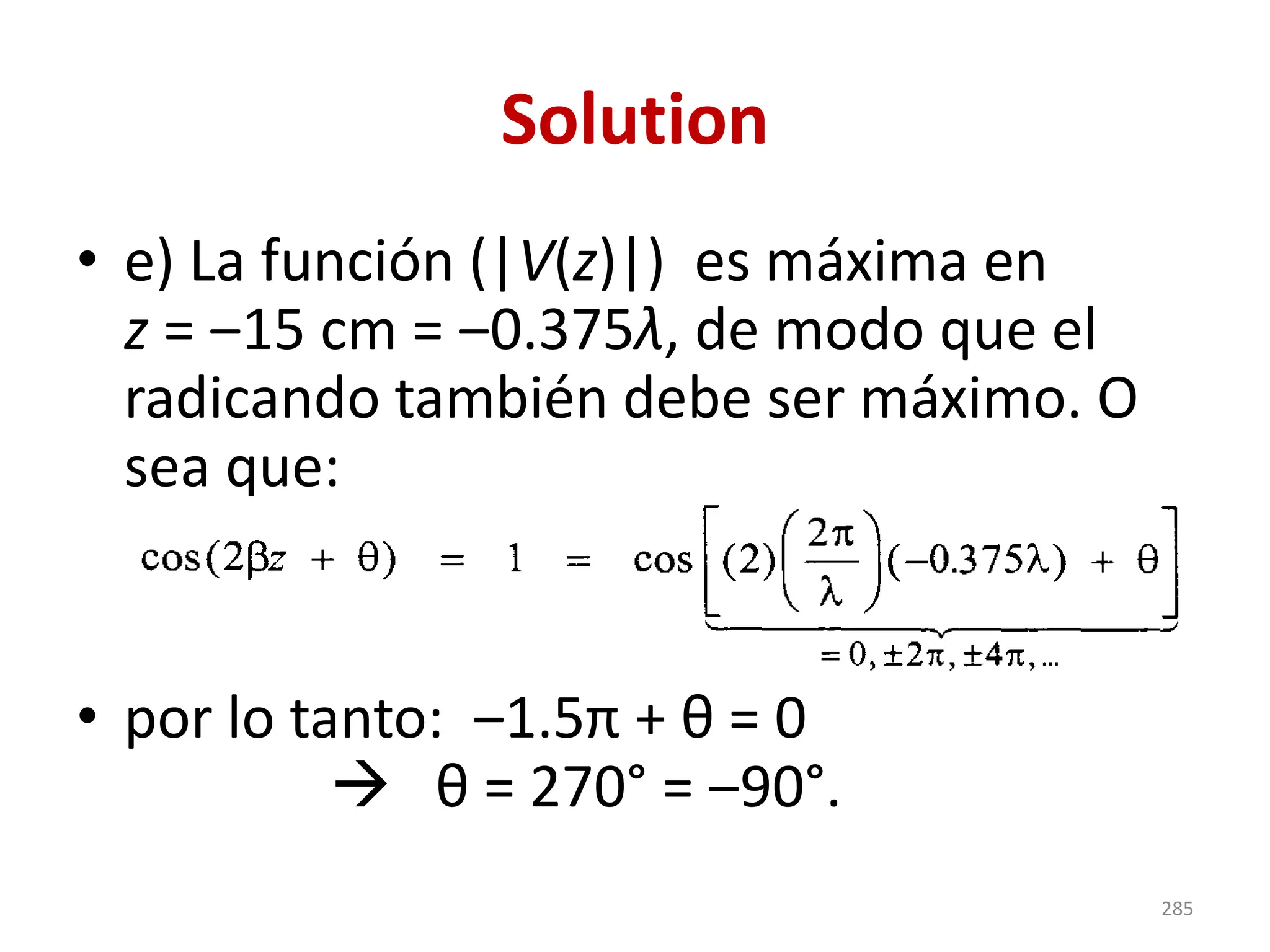
• e) Lafunción (|V(z)|) es máxima en
z = ‒15 cm = ‒0.375λ, de modo que el
radicando también debe ser máximo. O
sea que:
• por lo tanto: ‒1.5π + θ = 0
→ θ = 270° = ‒90°.
285
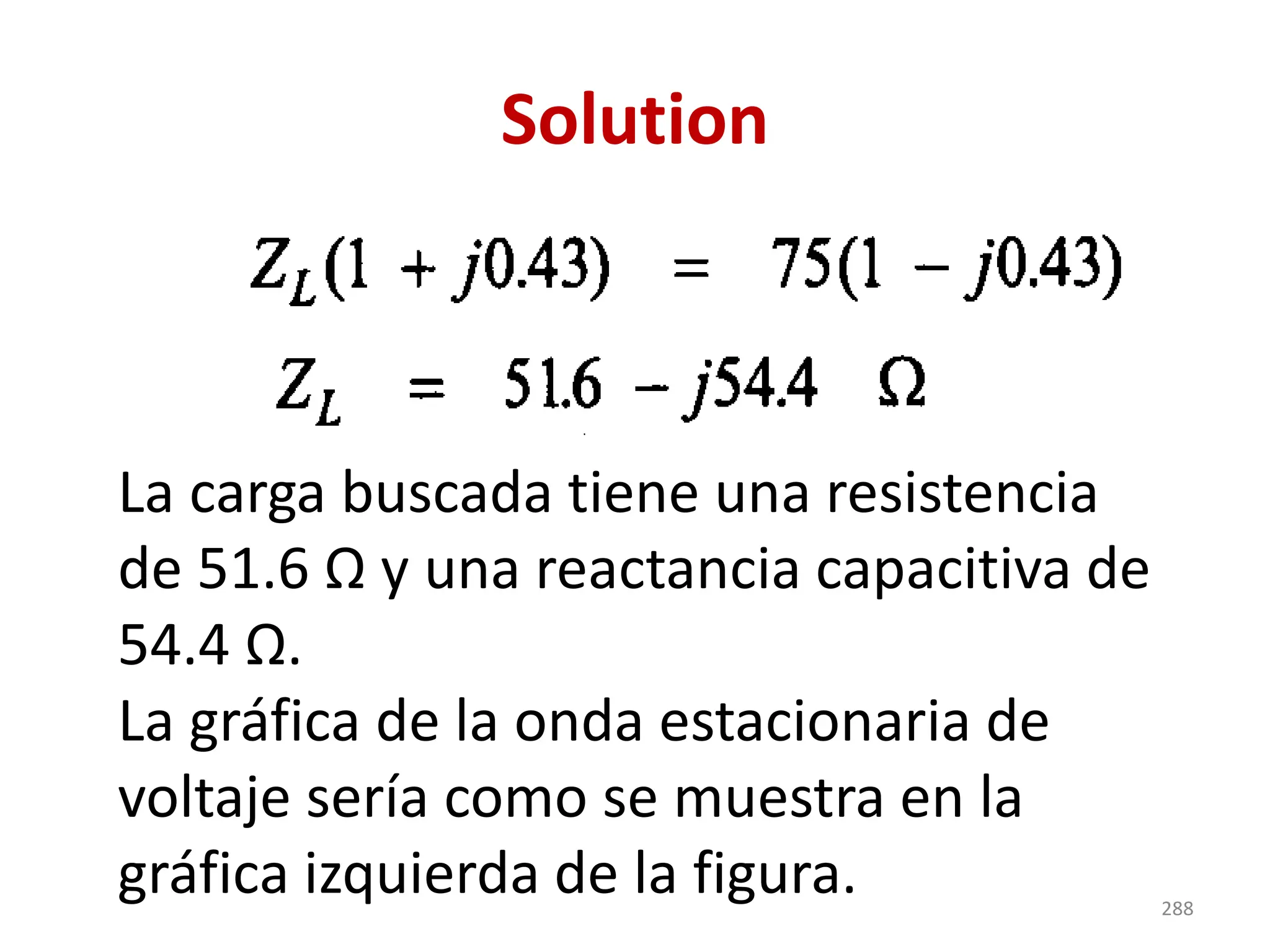
Solution
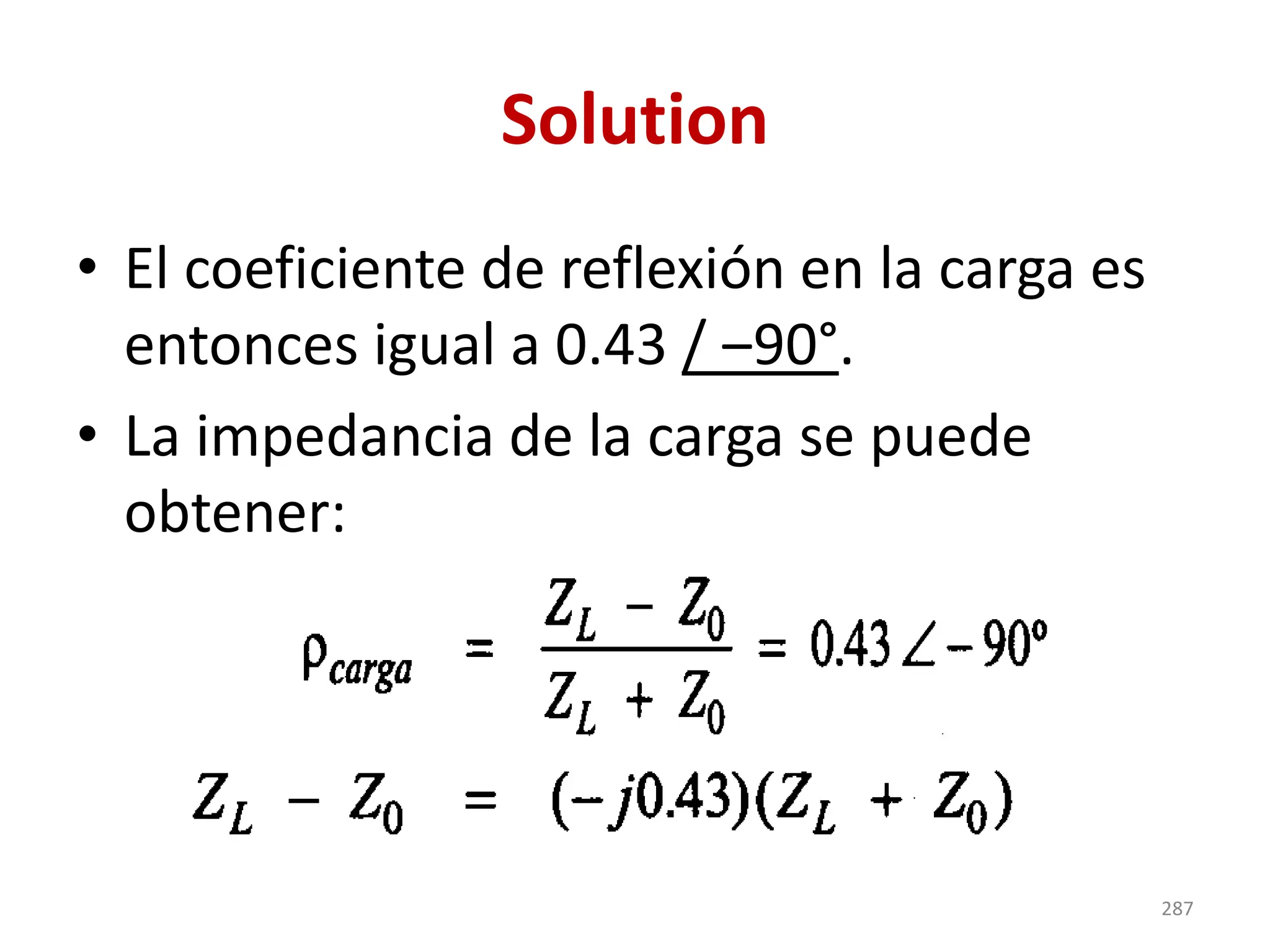
• El coeficientede reflexión en la carga es
entonces igual a 0.43 / ‒90°.
• La impedancia de la carga se puede
obtener:
287
288.
Solution
La carga buscadatiene una resistencia
de 51.6 Ω y una reactancia capacitiva de
54.4 Ω.
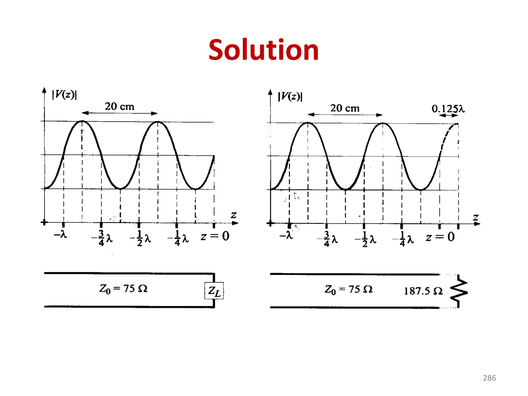
La gráfica de la onda estacionaria de
voltaje sería como se muestra en la
gráfica izquierda de la figura. 288
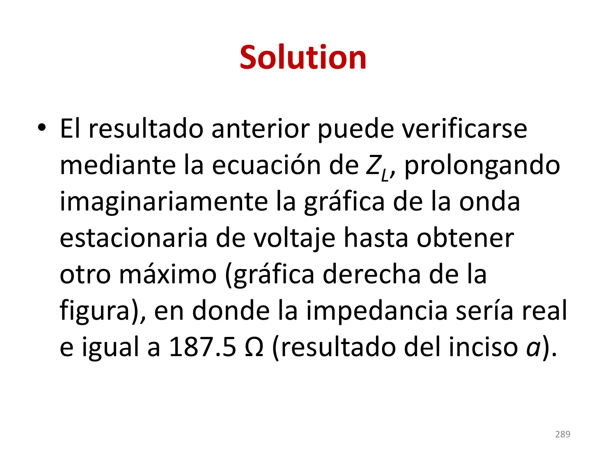
289.
Solution
• El resultadoanterior puede verificarse
mediante la ecuación de ZL, prolongando
imaginariamente la gráfica de la onda
estacionaria de voltaje hasta obtener
otro máximo (gráfica derecha de la
figura), en donde la impedancia sería real
e igual a 187.5 Ω (resultado del inciso a).
289
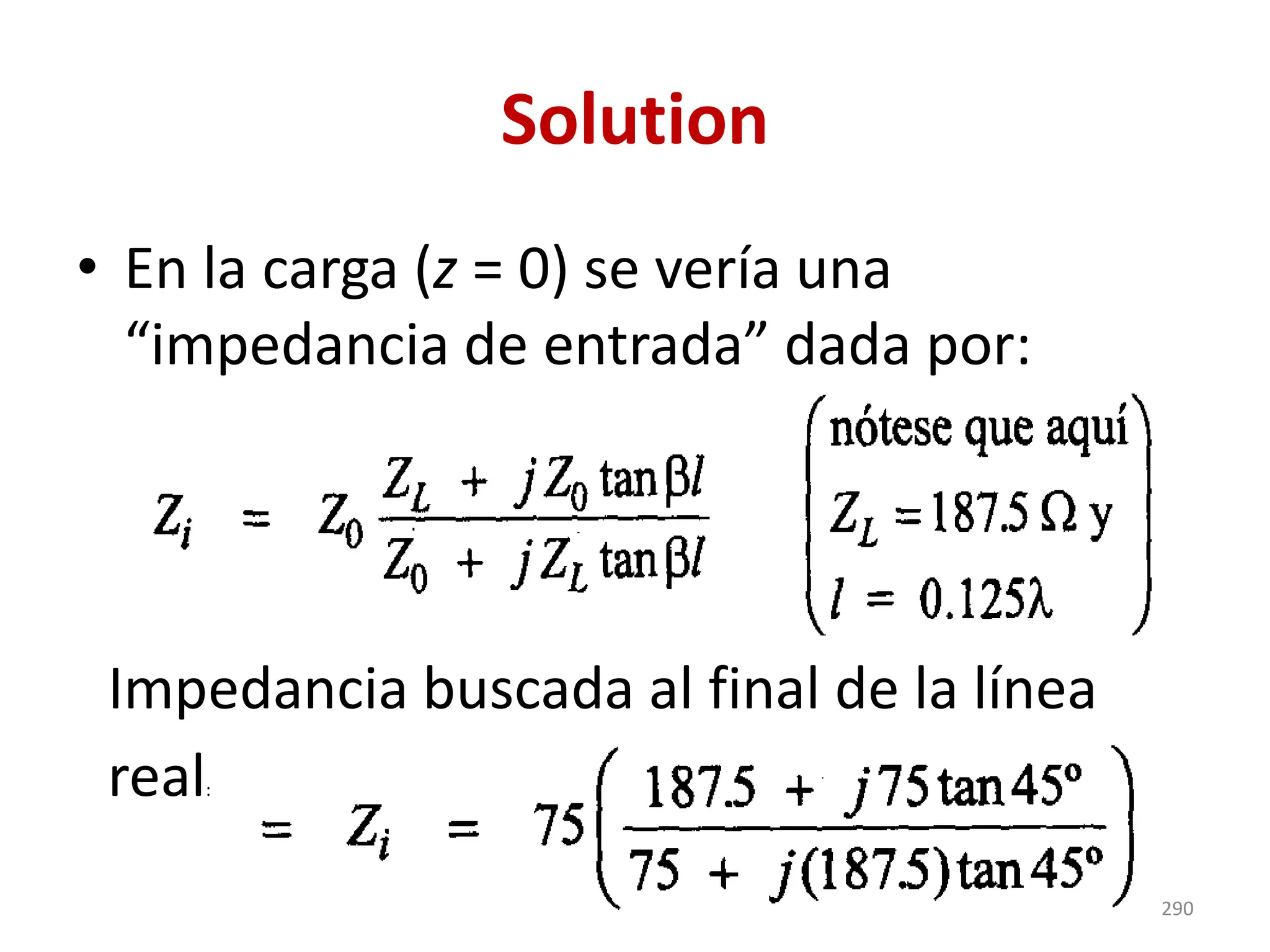
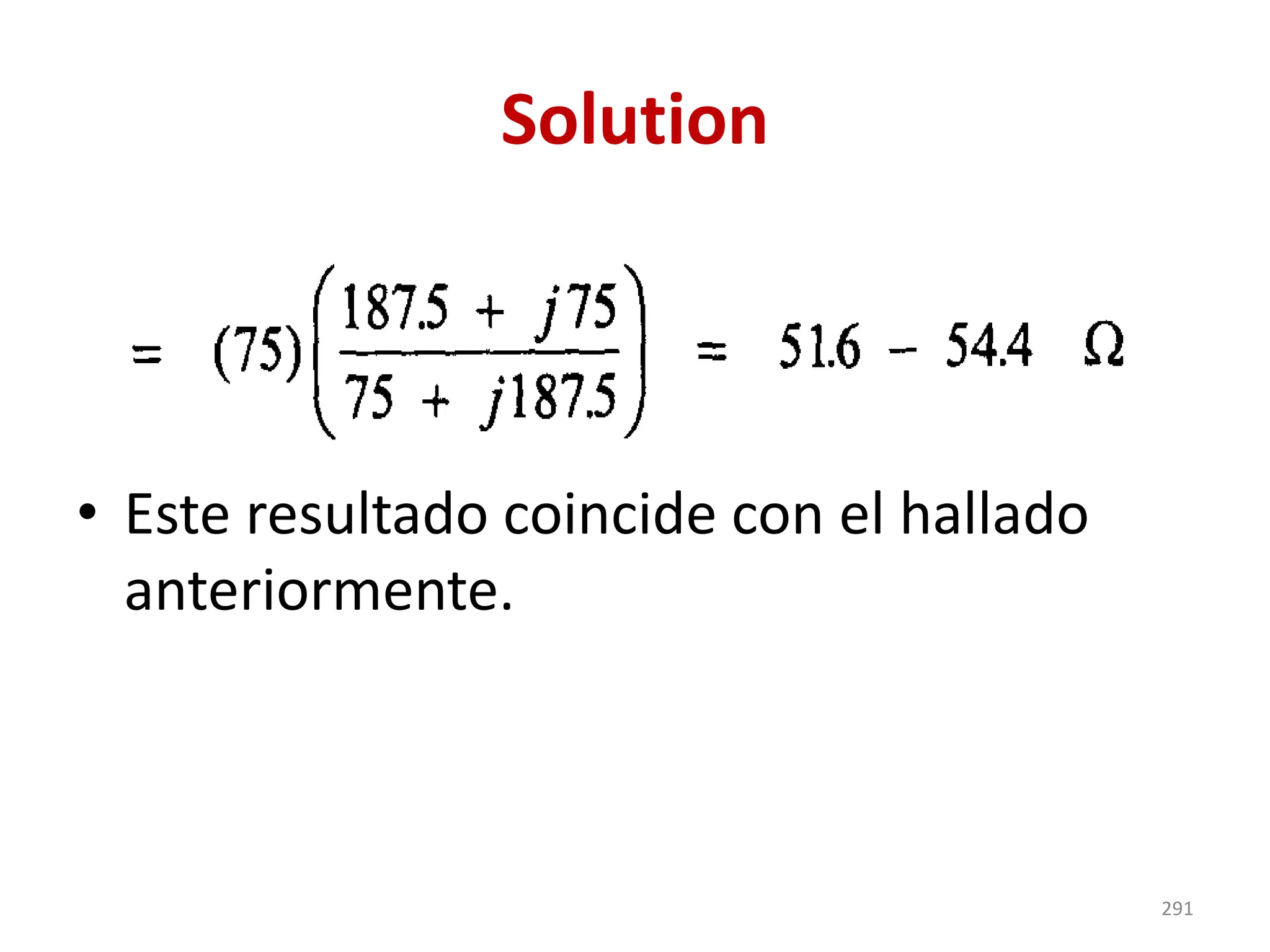
290.
Solution
• En lacarga (z = 0) se vería una
“impedancia de entrada” dada por:
Impedancia buscada al final de la línea
real:
290
Rule
• When theload is capacitive, the
standing voltage wave is upward
where the line ends.
• This is in line with the graph and the
results obtained in the previous
exercise.
292
293.
Rule
• On theother hand, if the load is
inductive, at the end of the line
there will be a descending voltage
wave.
293
294.
Reflections on thegenerator
• El generador es la fuente original de
las ondas de voltaje y corriente que
viajan a lo largo de la línea hacia la
carga.
• El generador tiene una impedancia
interna, Zg, que se combina en serie
con la impedancia de entrada de la
línea cuando ambos se conectan.
294
295.
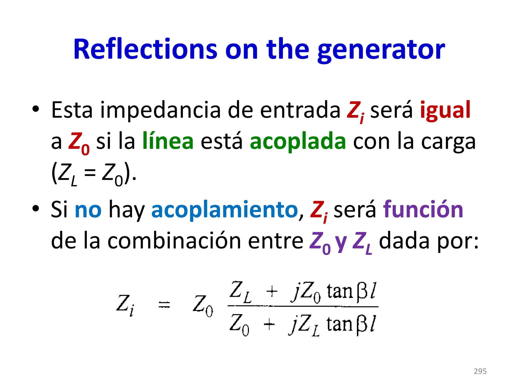
Reflections on thegenerator
• Esta impedancia de entrada Zi será igual
a Z0 si la línea está acoplada con la carga
(ZL = Z0).
• Si no hay acoplamiento, Zi será función
de la combinación entre Z0 y ZL dada por:
295
296.
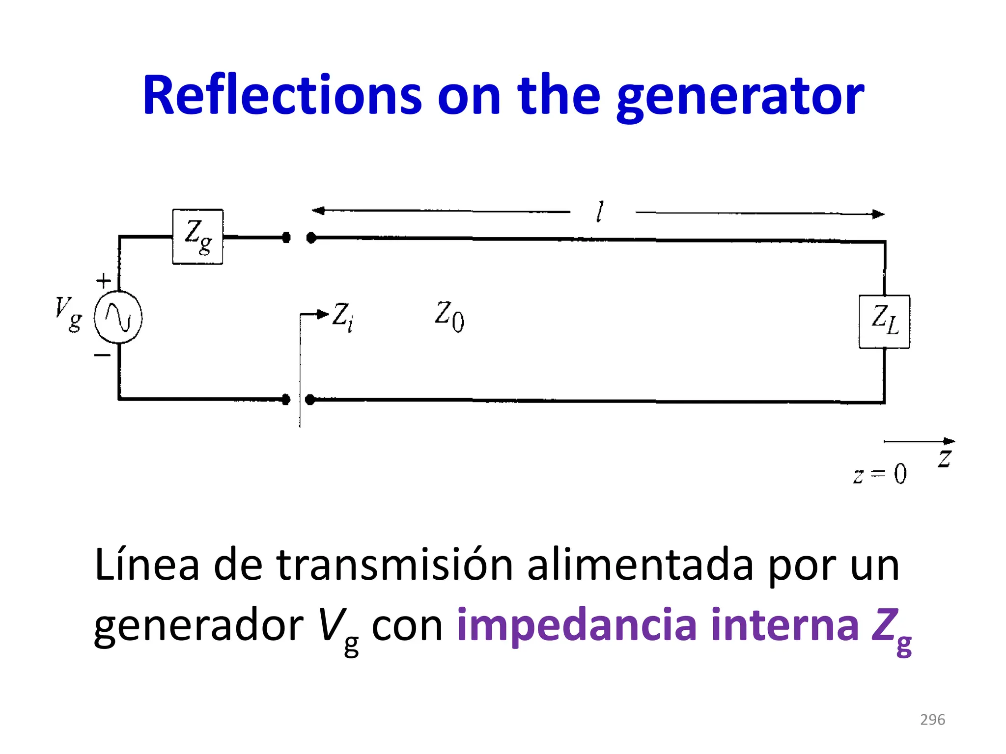
Reflections on thegenerator
Línea de transmisión alimentada por un
generador Vg con impedancia interna Zg
296
297.
Reflections on thegenerator
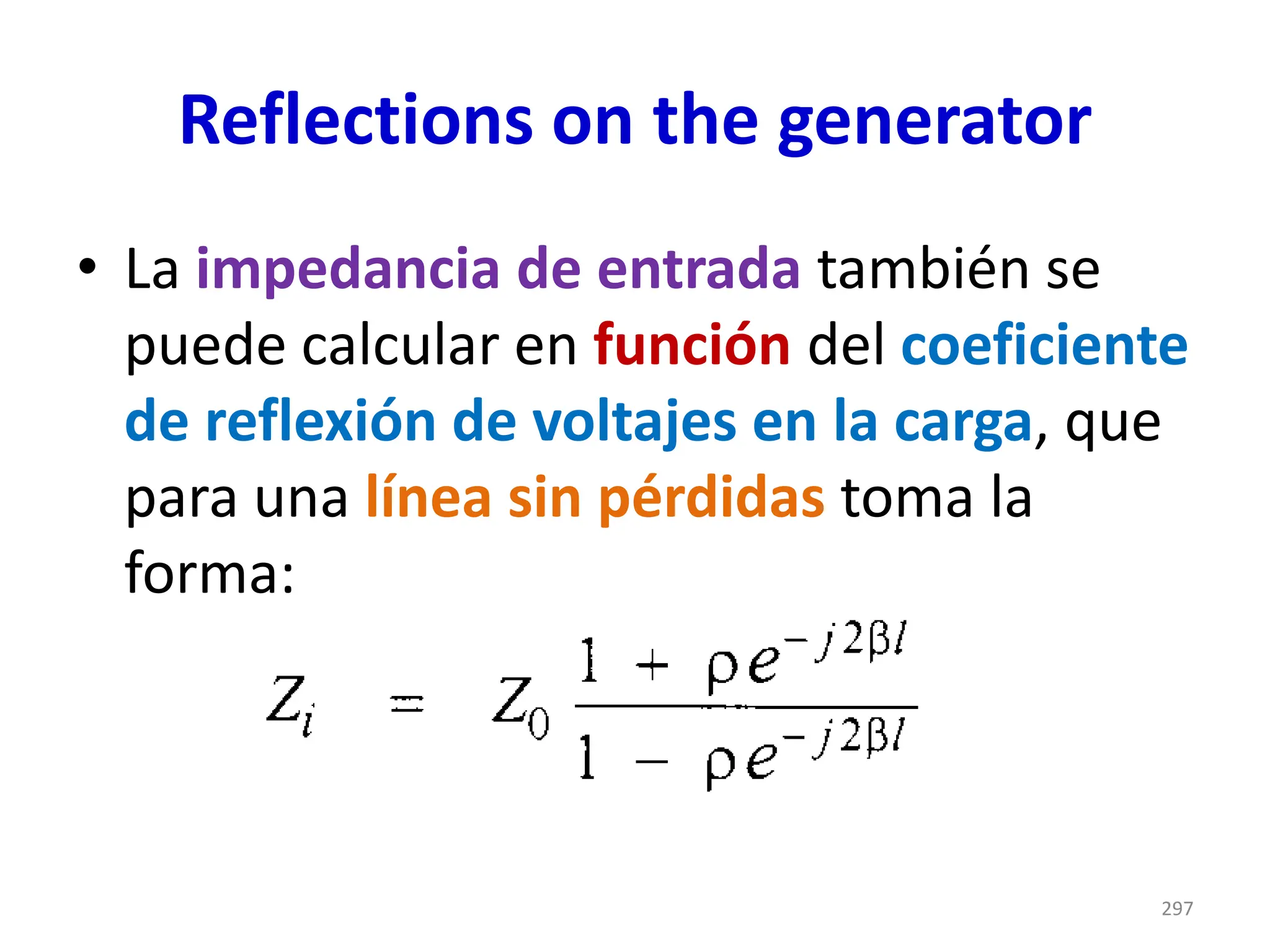
• La impedancia de entrada también se
puede calcular en función del coeficiente
de reflexión de voltajes en la carga, que
para una línea sin pérdidas toma la
forma:
297
298.
Reflections on thegenerator
• En la fórmula anterior se observa que el
término ρe‒j2βl es el coeficiente de
reflexión trasladado al punto inicial de
la línea para z = ‒l.
298
299.
Reflections on thegenerator
• Supóngase que una onda reflejada en la
carga (debido a que ZL ≠ Z0) se dirige de
regreso al generador.
• Si Zg (que se convierte en la nueva carga)
≠ Z0, habrá un coeficiente de reflexión en
la entrada de la línea, dando origen a una
segunda onda que se dirigirá hacia la
carga ZL, y así sucesivamente.
299
300.
Reflections on thegenerator
• Este proceso podría durar
indefinidamente, y la onda estacionaria
final sería la superposición de todas las
ondas producidas.
• Este efecto se reduce en la práctica
debido a que α ≠ 0 y la amplitud de las
ondas reflejadas disminuye de acuerdo
con e‒αl en cada sentido.
300
301.
Reflections on thegenerator
• Es común que el valor de Zg sea muy
cercano o igual al de Z0 (generador
acoplado con la línea).
• Esto hace que la onda reflejada en el
generador sea despreciable o casi
nula.
301
302.
Reflections on thegenerator
Conclusión:
• La conexión ideal para que se le
entregue máxima potencia a la línea y no
haya reflexiones, es que Zg = Z0 = ZL.
• La potencia entregada a la línea (Pi), es
la mitad de la potencia total original, y si
α ≈ 0, la potencia entregada a la carga es
prácticamente igual a Pi.
302
La matriz detransmisión
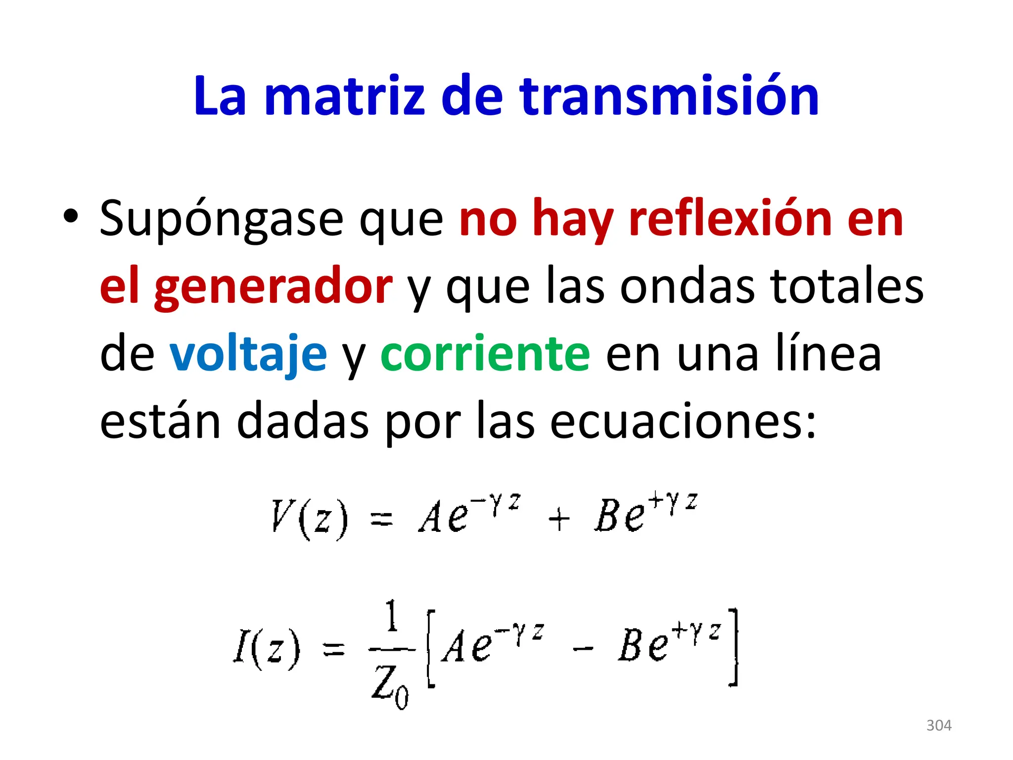
• Supóngase que no hay reflexión en
el generador y que las ondas totales
de voltaje y corriente en una línea
están dadas por las ecuaciones:
304
305.
La matriz detransmisión
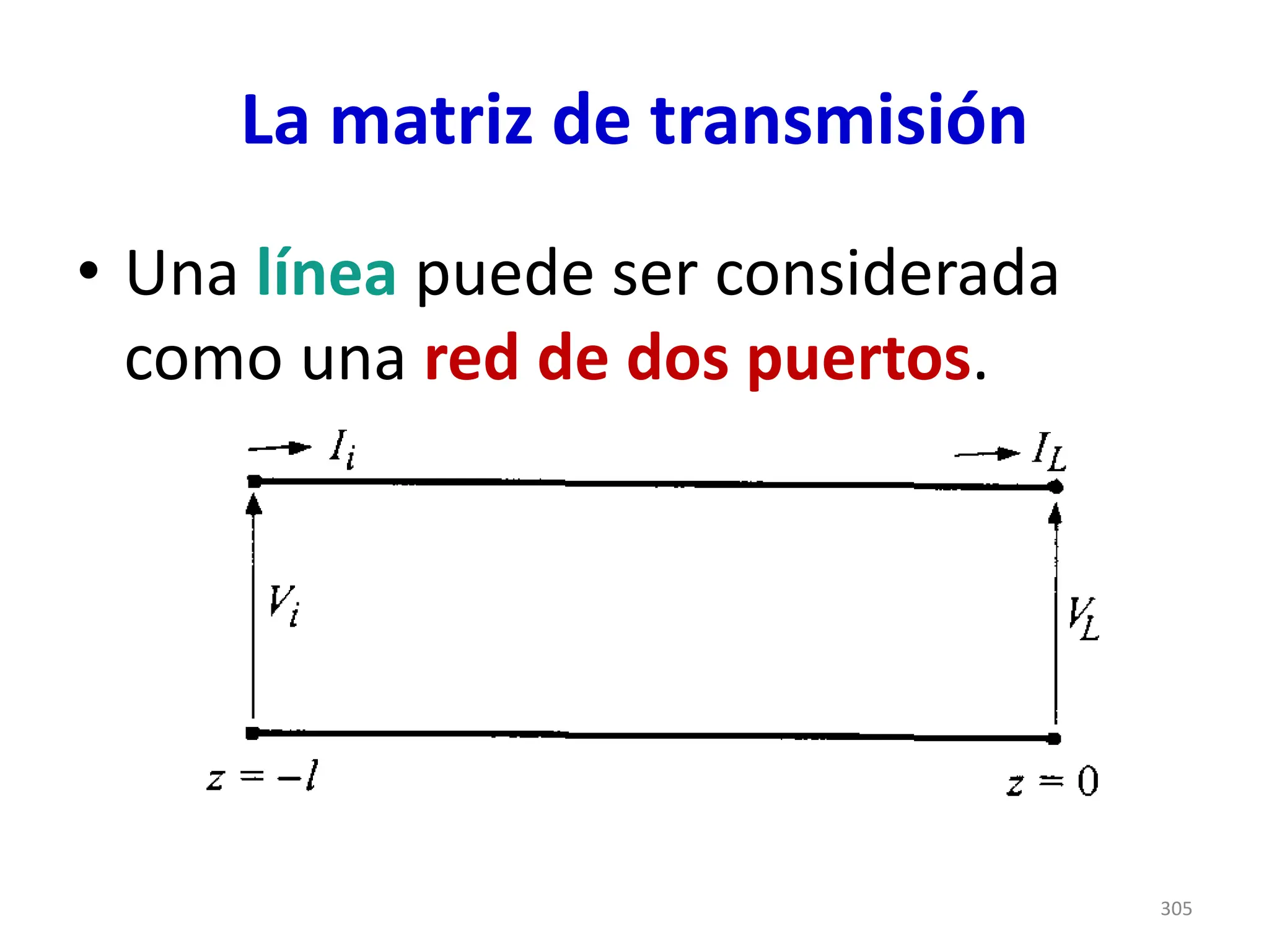
• Una línea puede ser considerada
como una red de dos puertos.
305
306.
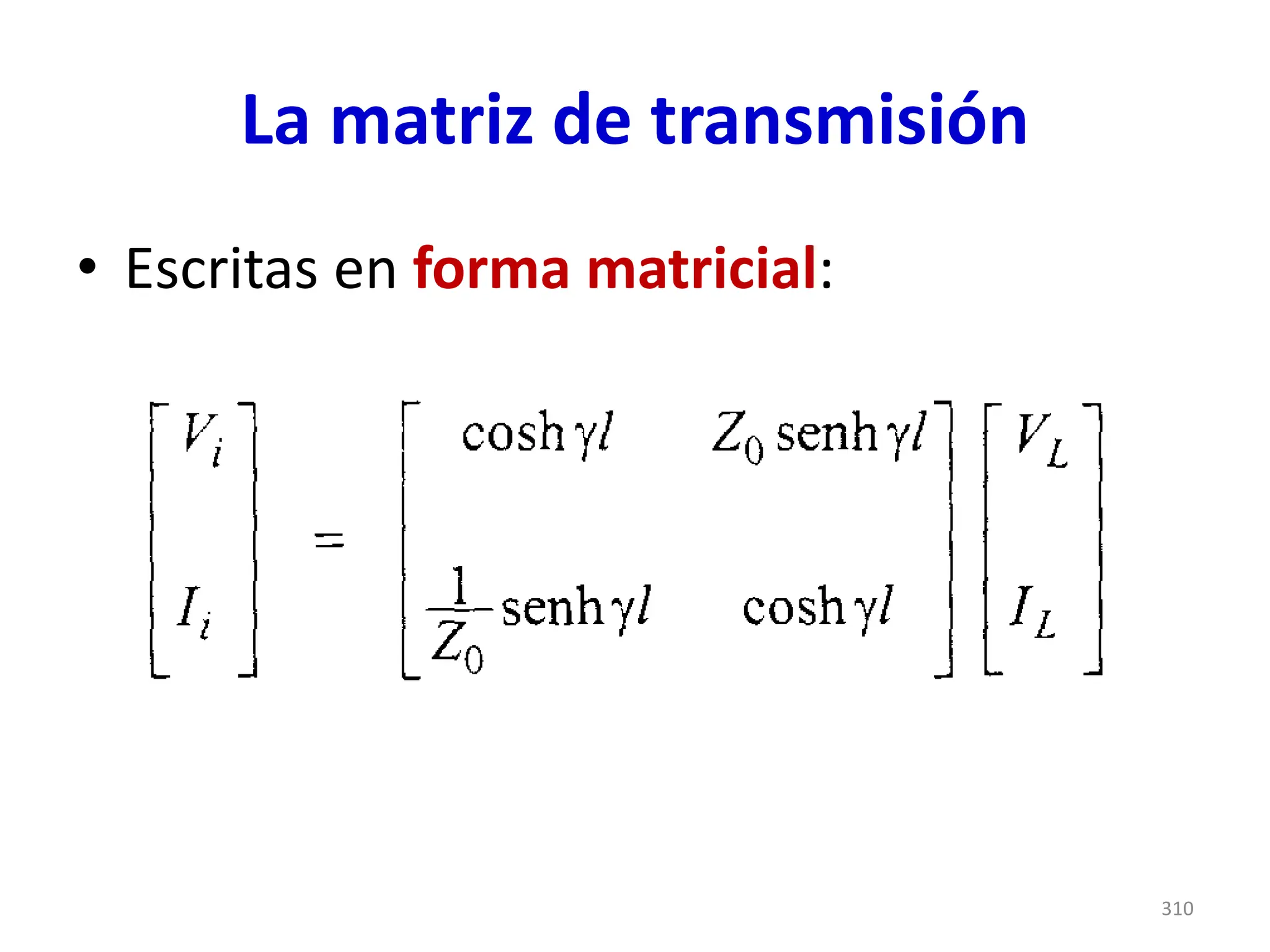
La matriz detransmisión
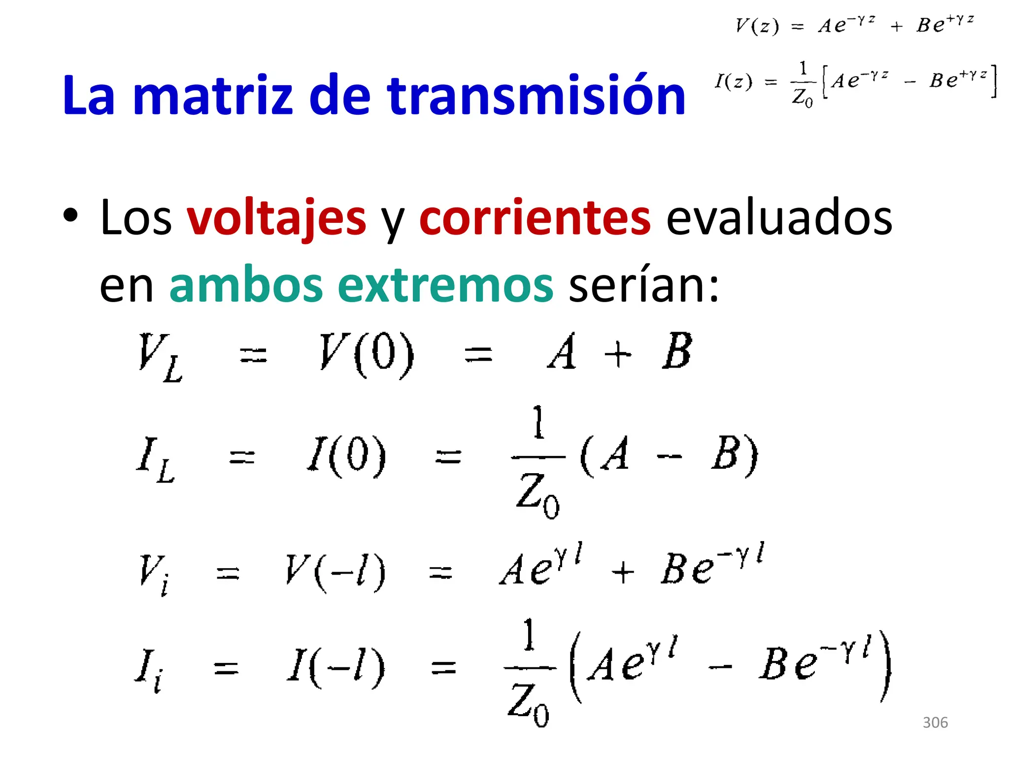
• Los voltajes y corrientes evaluados
en ambos extremos serían:
306
307.
La matriz detransmisión
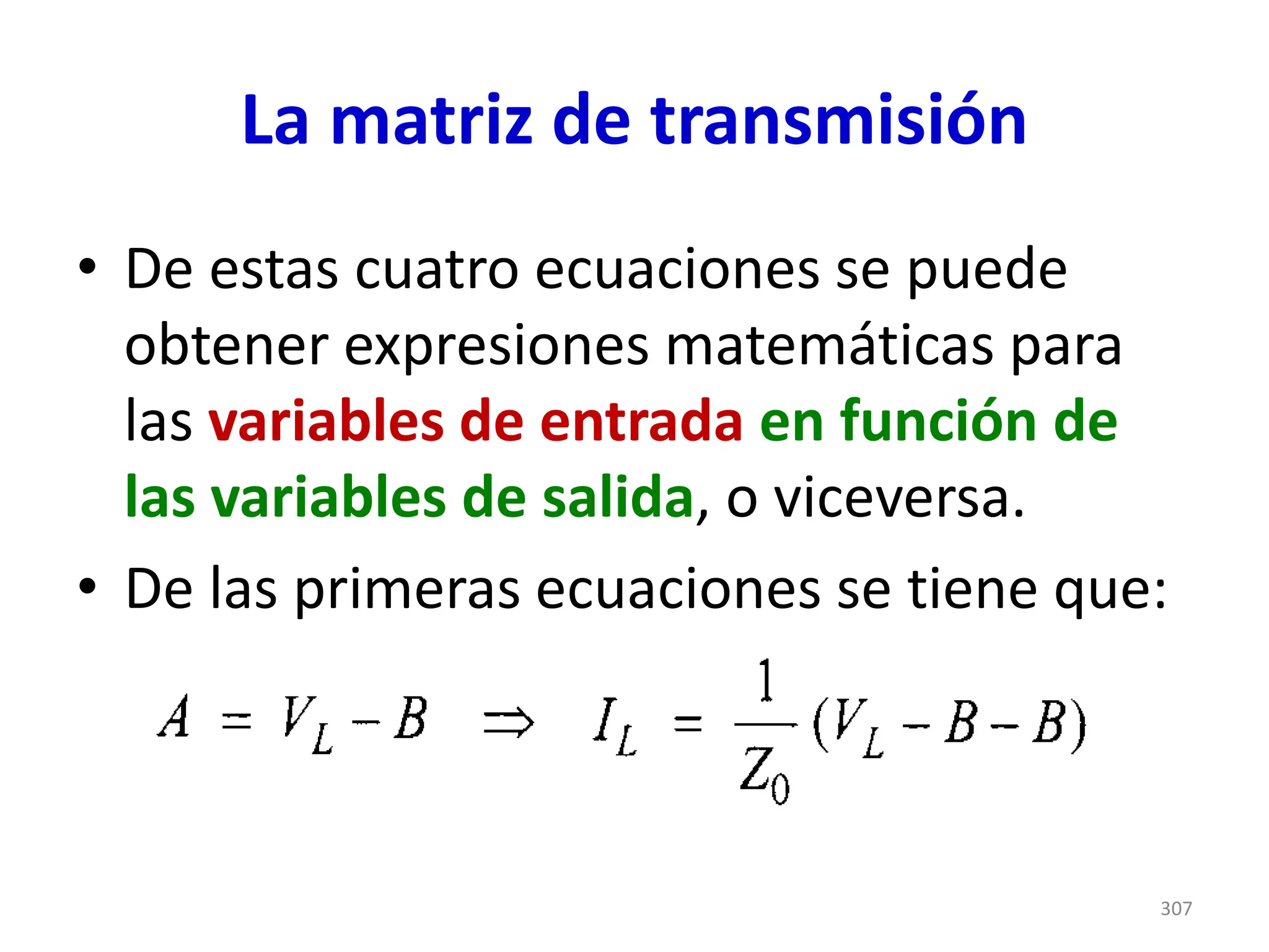
• De estas cuatro ecuaciones se puede
obtener expresiones matemáticas para
las variables de entrada en función de
las variables de salida, o viceversa.
• De las primeras ecuaciones se tiene que:
307
308.
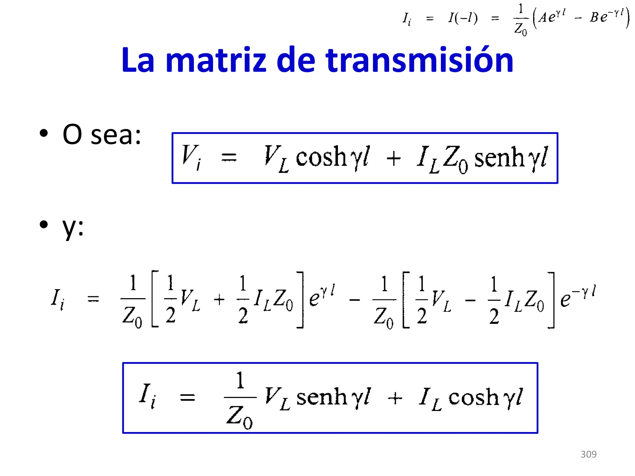
La matriz detransmisión
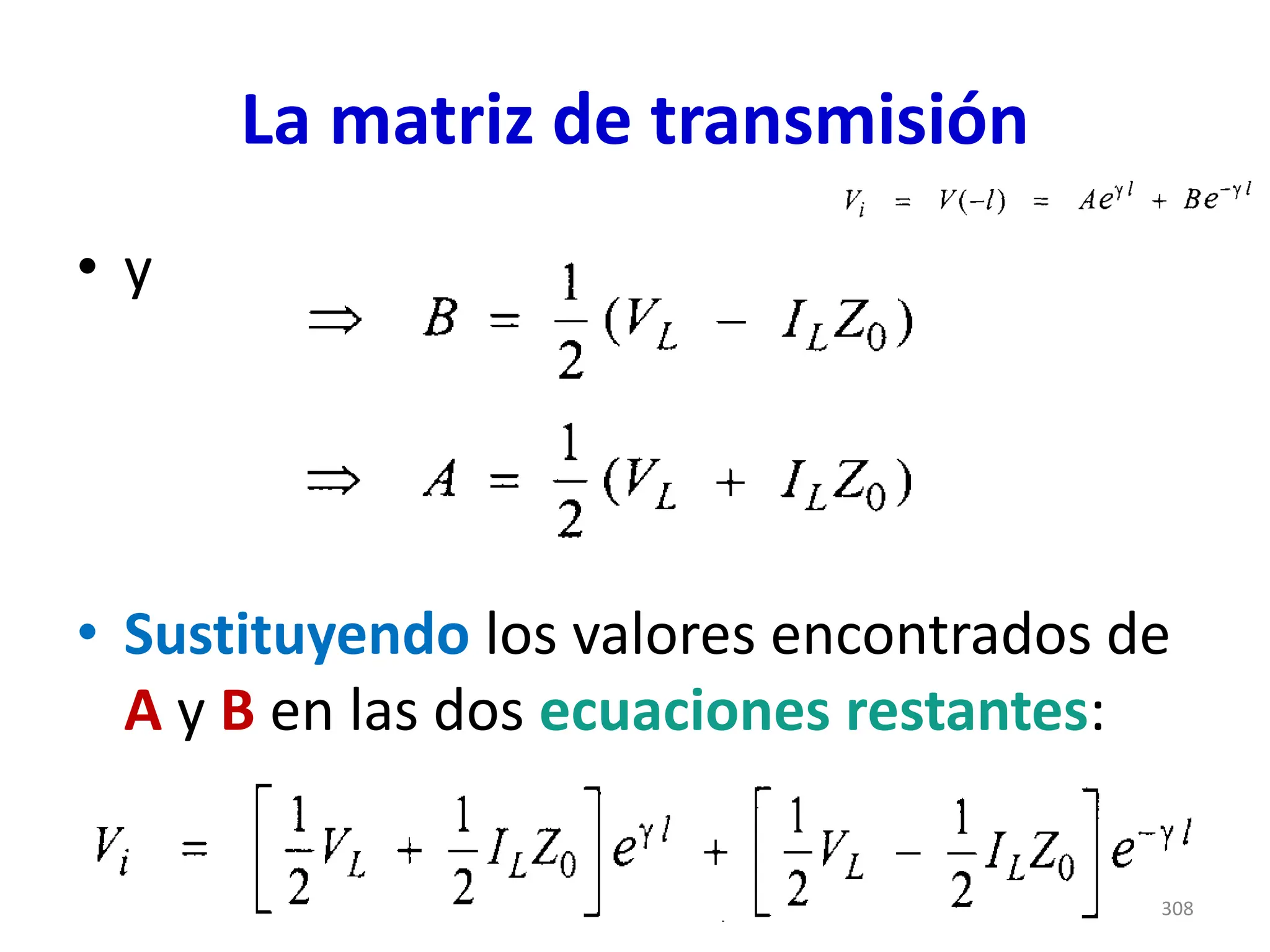
• y
• Sustituyendo los valores encontrados de
A y B en las dos ecuaciones restantes:
308
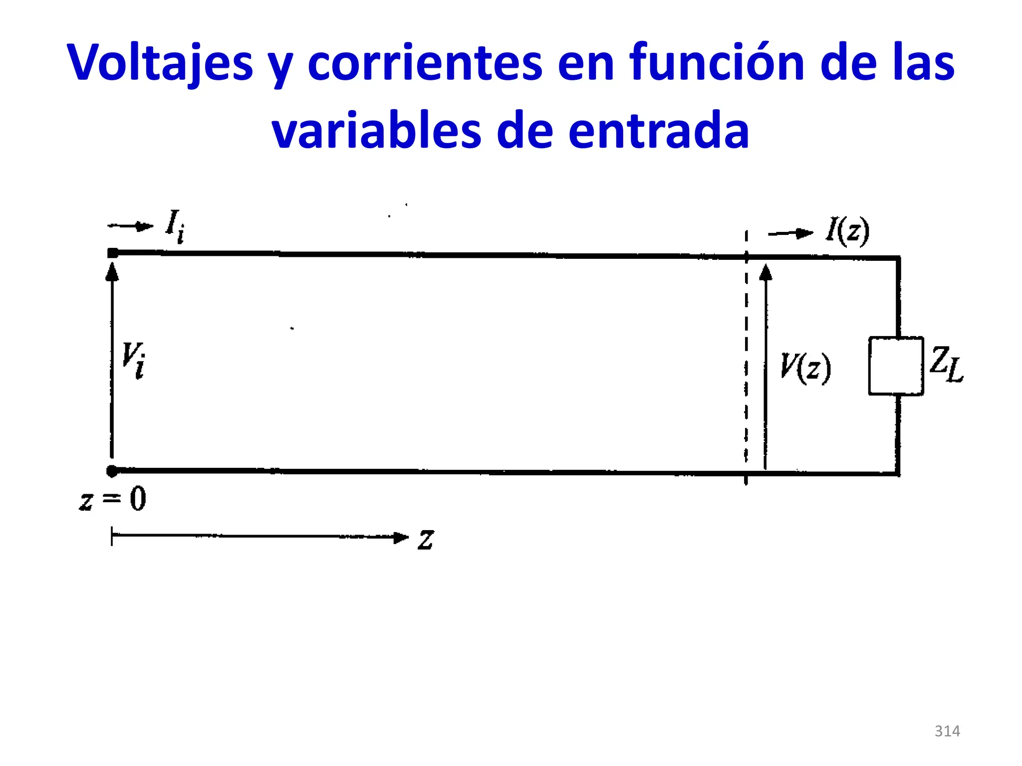
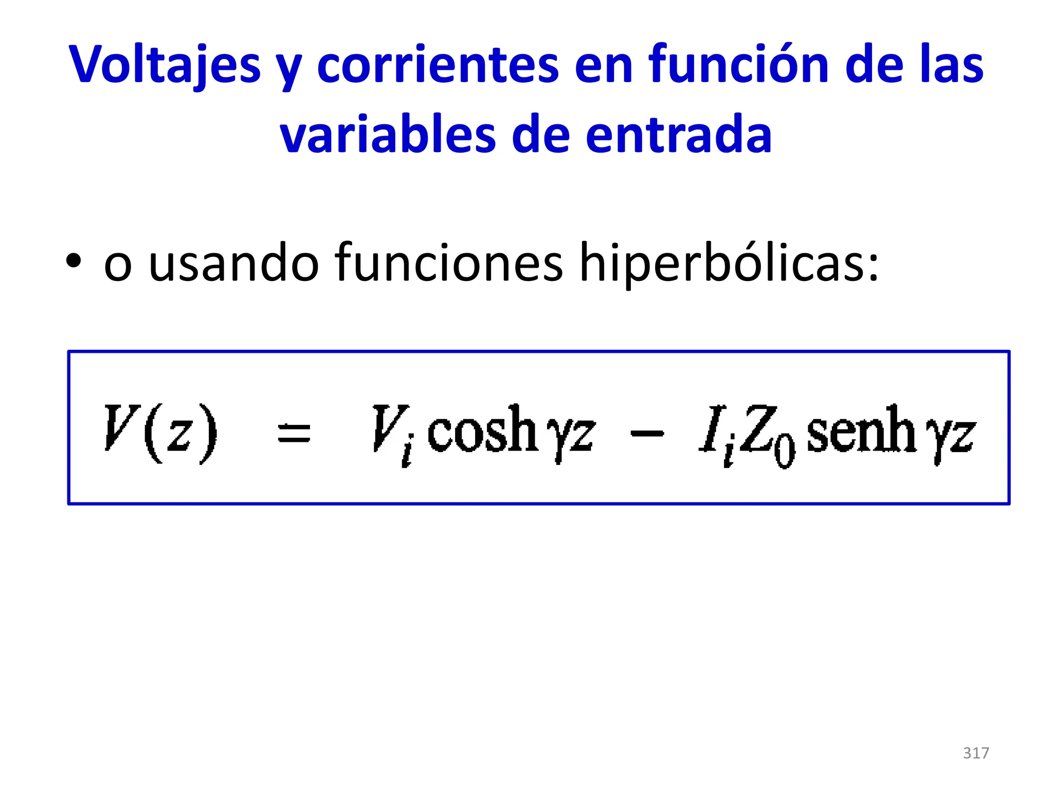
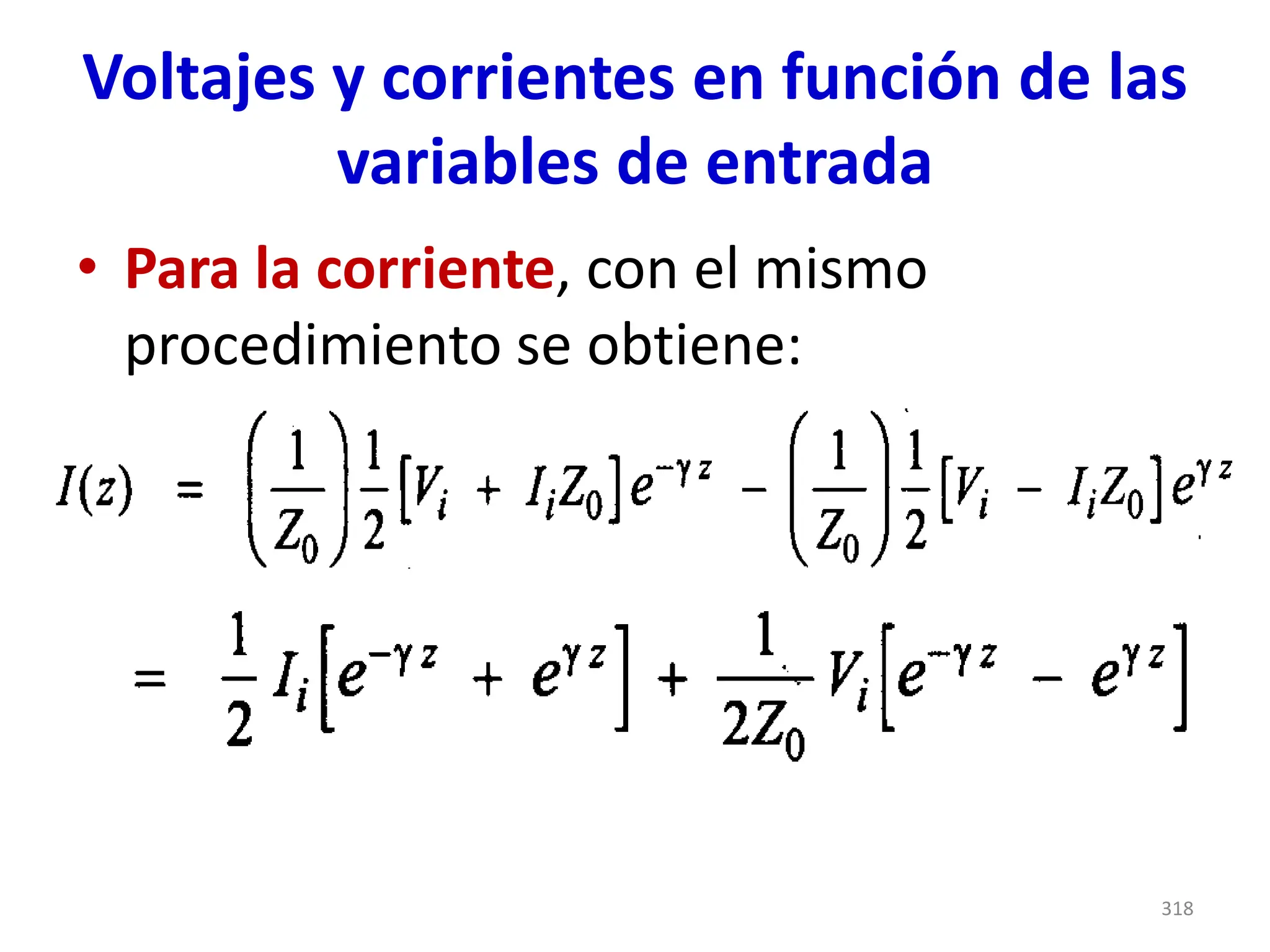
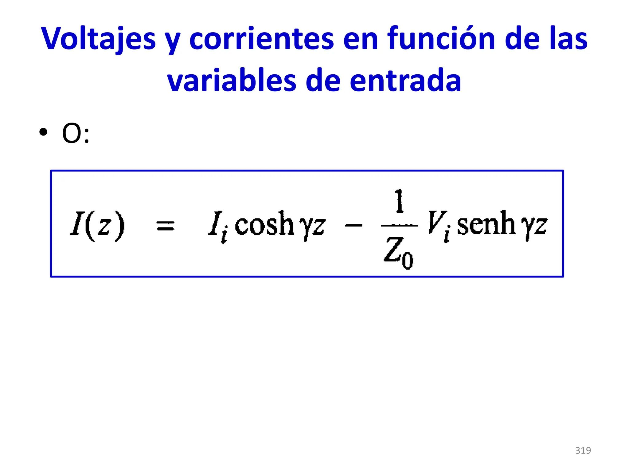
Voltajes y corrientesen función de las
variables de entrada
• También es posible obtener expresiones
para el voltaje y la corriente en cualquier
punto de la línea en función de las
variables de entrada, (Vi e Ii).
• Para esto, conviene tomar ahora z = 0 en
donde la línea comienza.
313
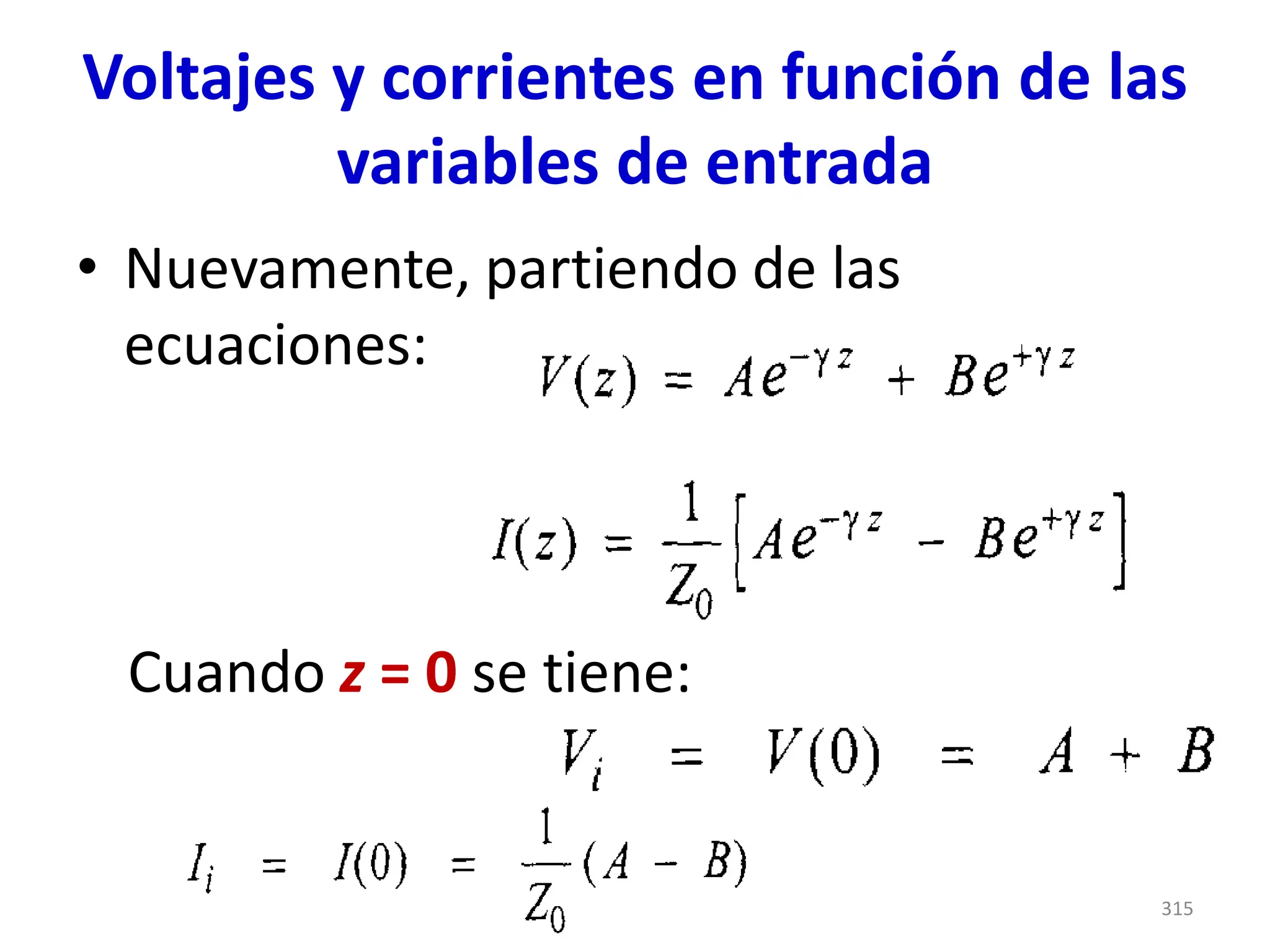
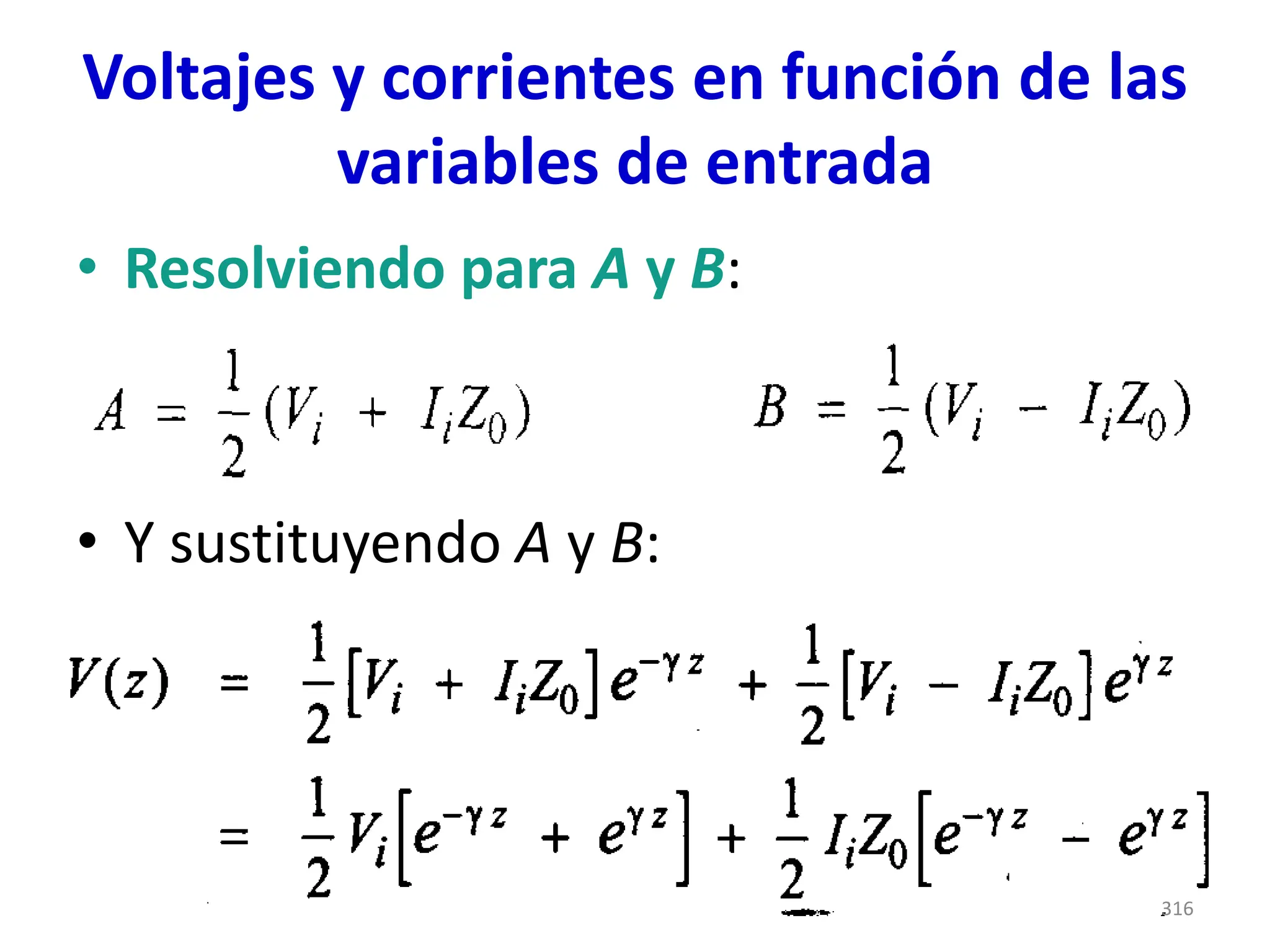
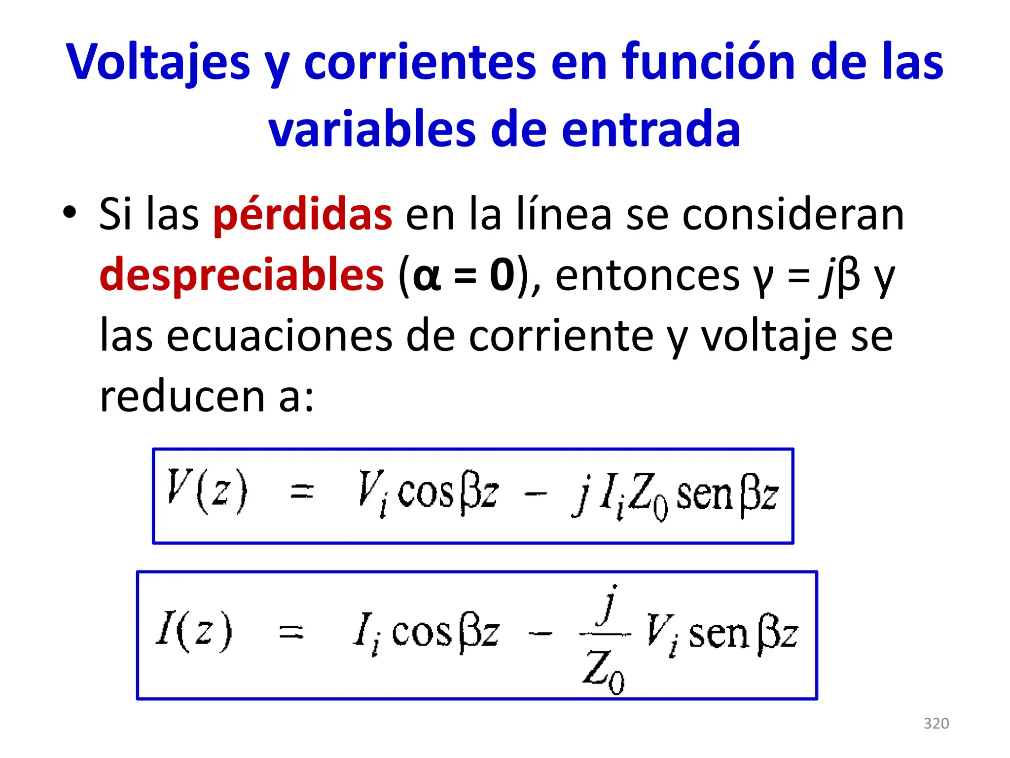
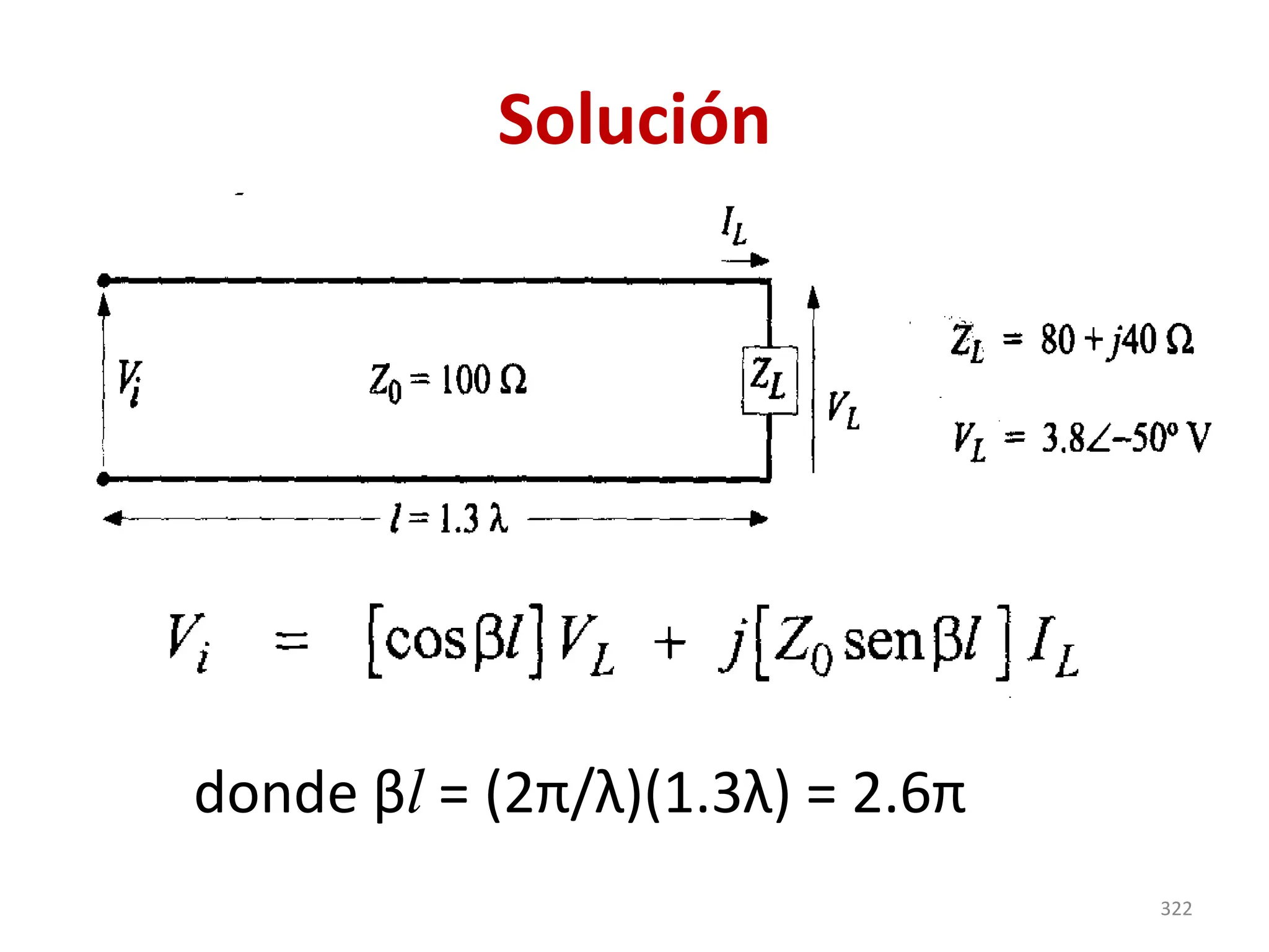
Voltajes y corrientesen función de las
variables de entrada
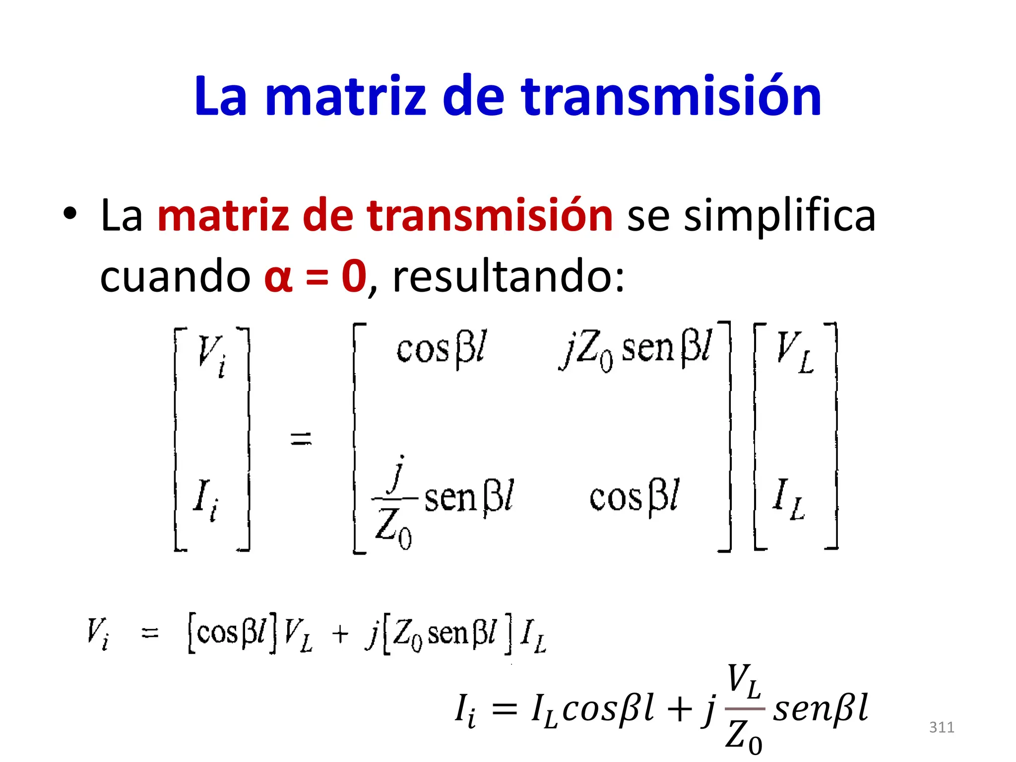
• Si las pérdidas en la línea se consideran
despreciables (α = 0), entonces γ = jβ y
las ecuaciones de corriente y voltaje se
reducen a:
320
321.
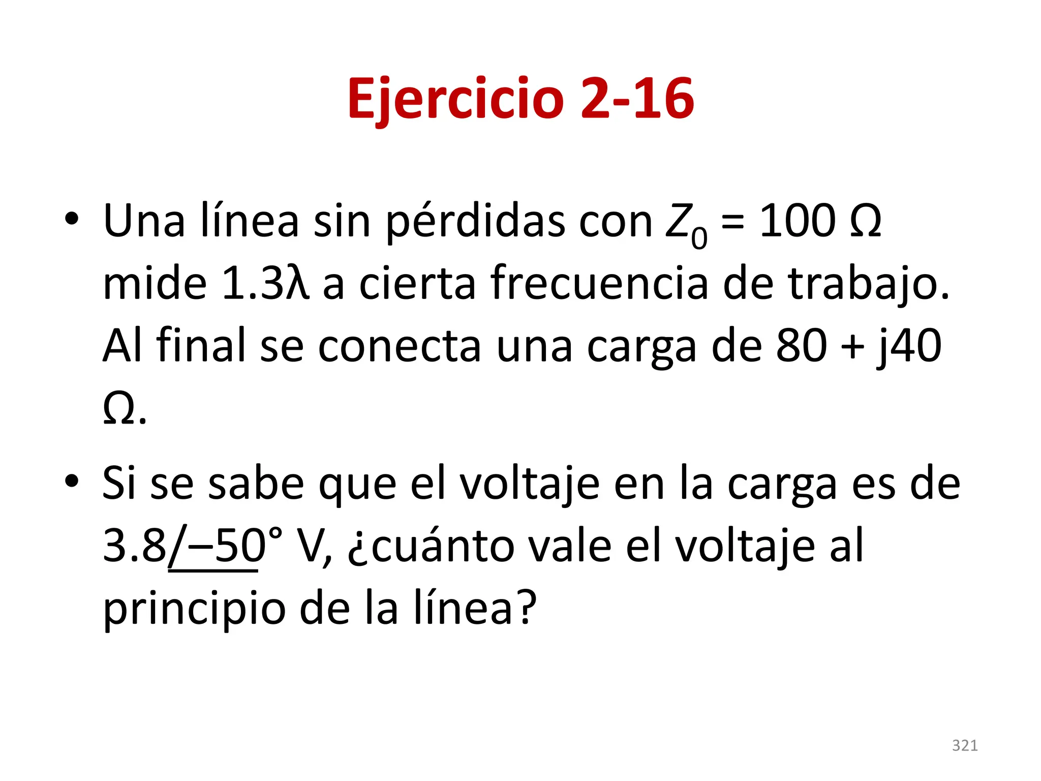
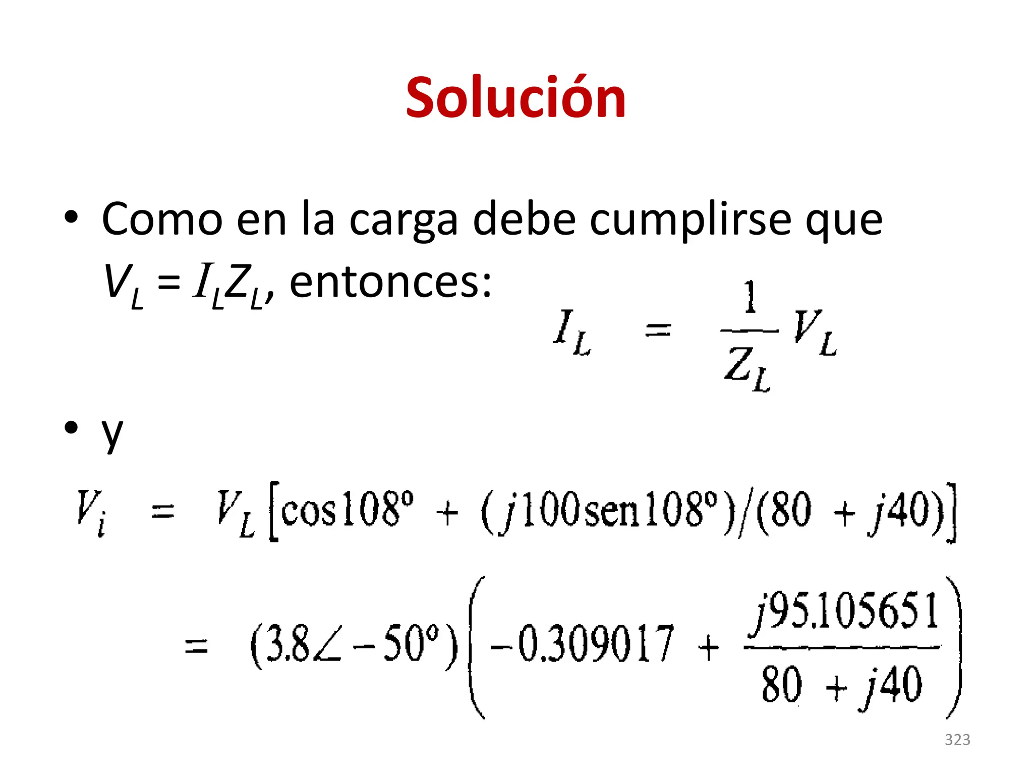
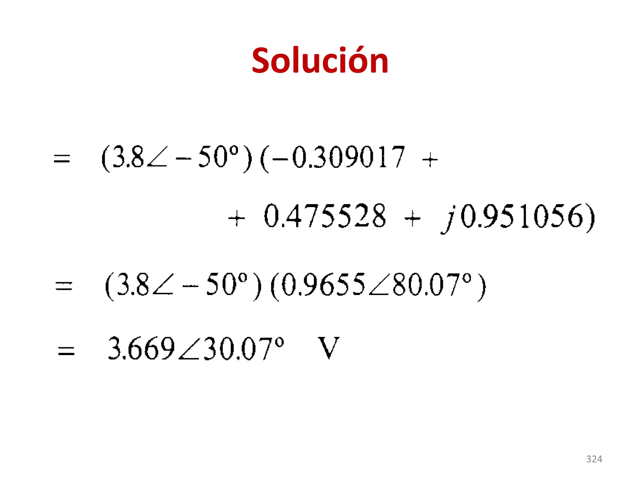
Ejercicio 2-16
• Unalínea sin pérdidas con Z0 = 100 Ω
mide 1.3λ a cierta frecuencia de trabajo.
Al final se conecta una carga de 80 + j40
Ω.
• Si se sabe que el voltaje en la carga es de
3.8/‒50° V, ¿cuánto vale el voltaje al
principio de la línea?
321
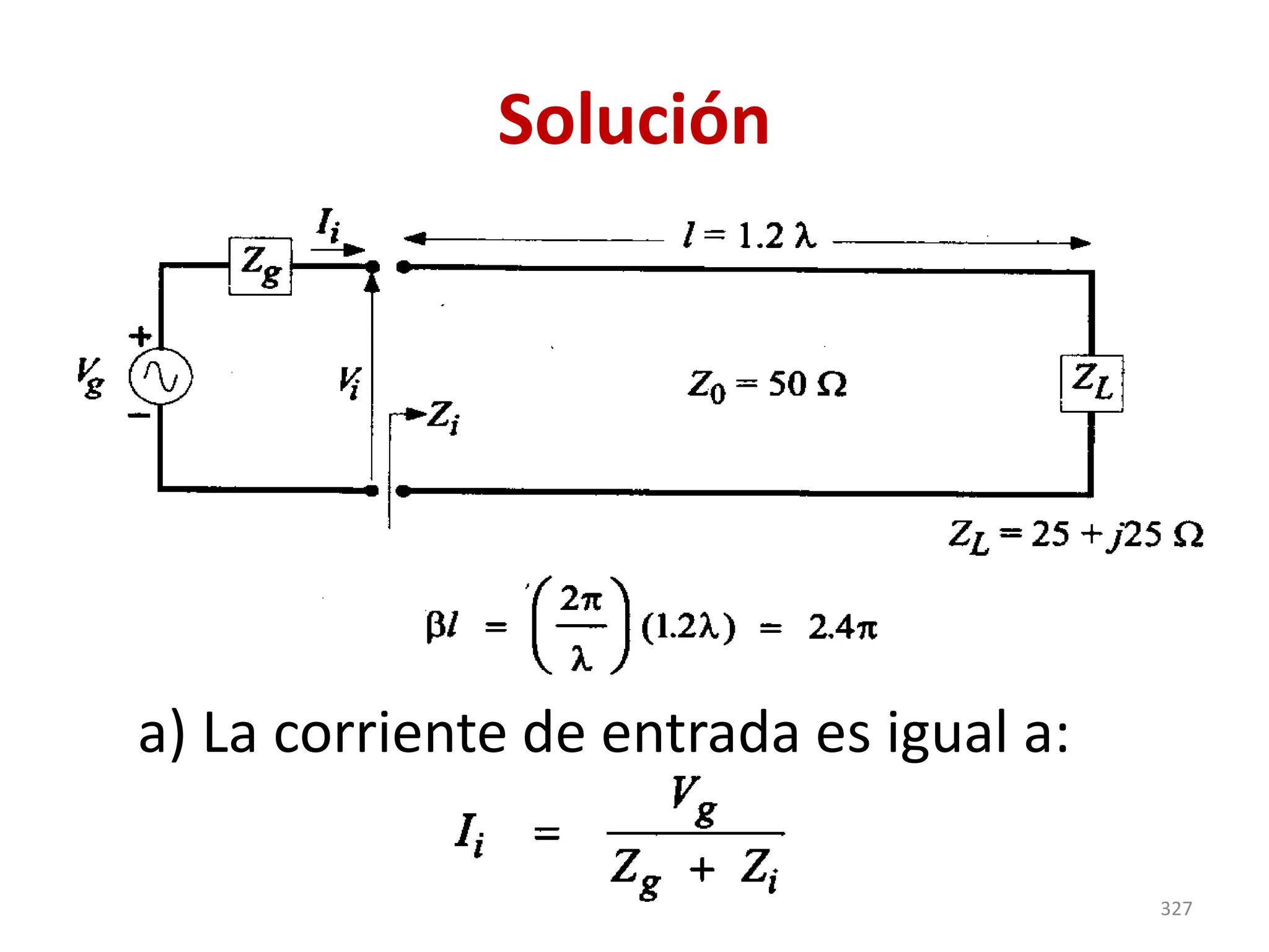
Ejercicio 2.17
• Unalínea sin pérdidas con Z0 = 50 Ω mide
1.2 λ a cierta frecuencia de trabajo.
• La línea es alimentada por un generador
con Vg = 15 /0° V, cuya resistencia interna
es igual a 50 Ω. Al final de la línea hay
una carga de 25 + j25 Ω.
325
326.
Ejercicio 2.17
Encuentre:
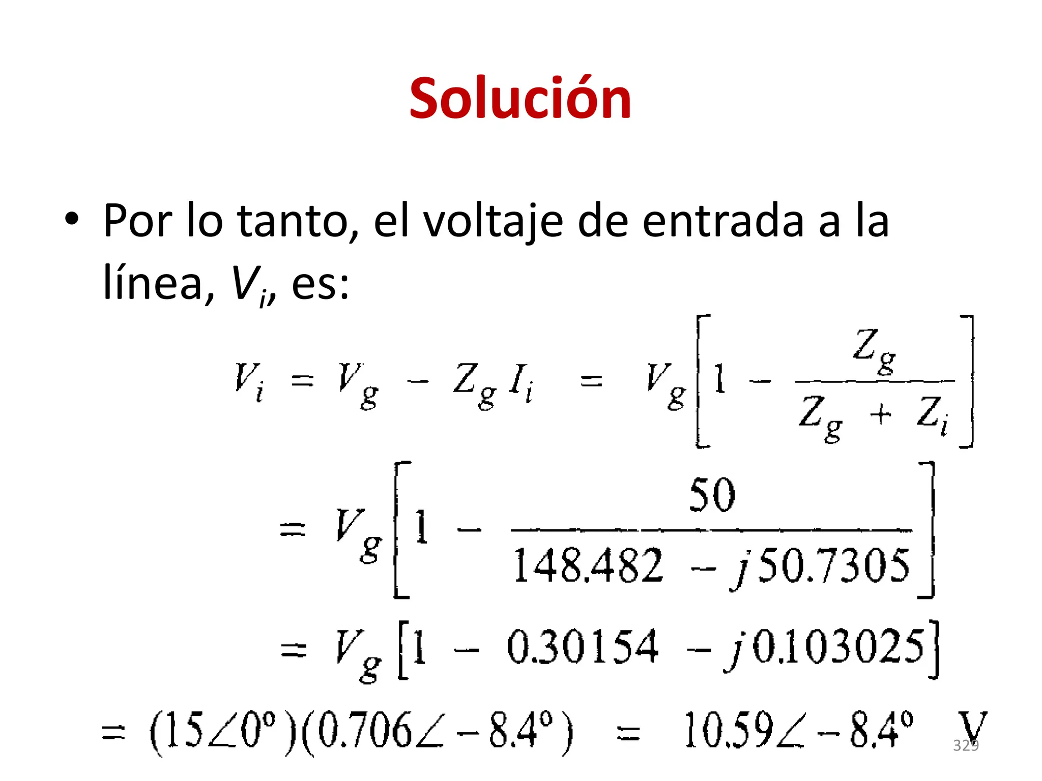
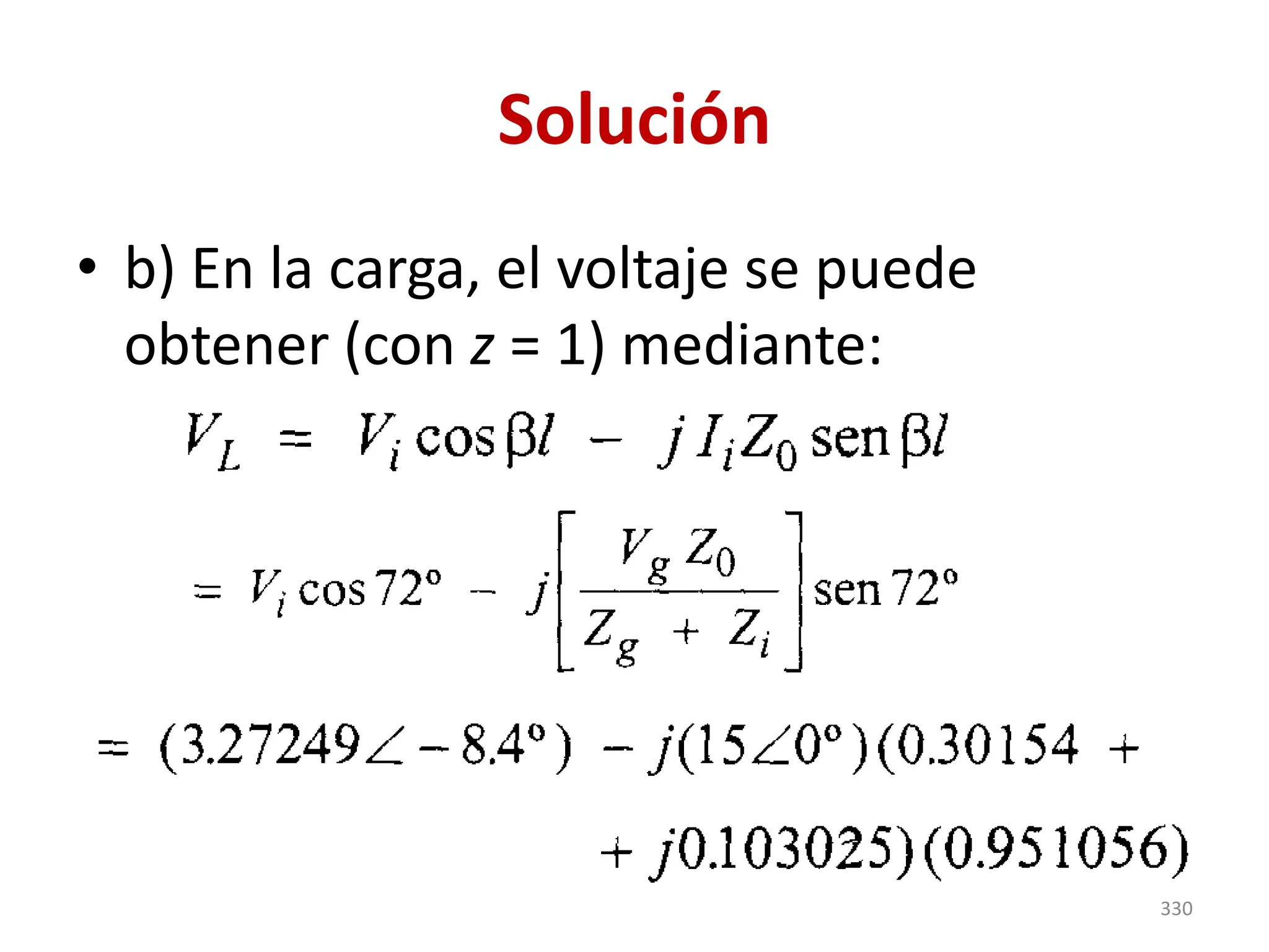
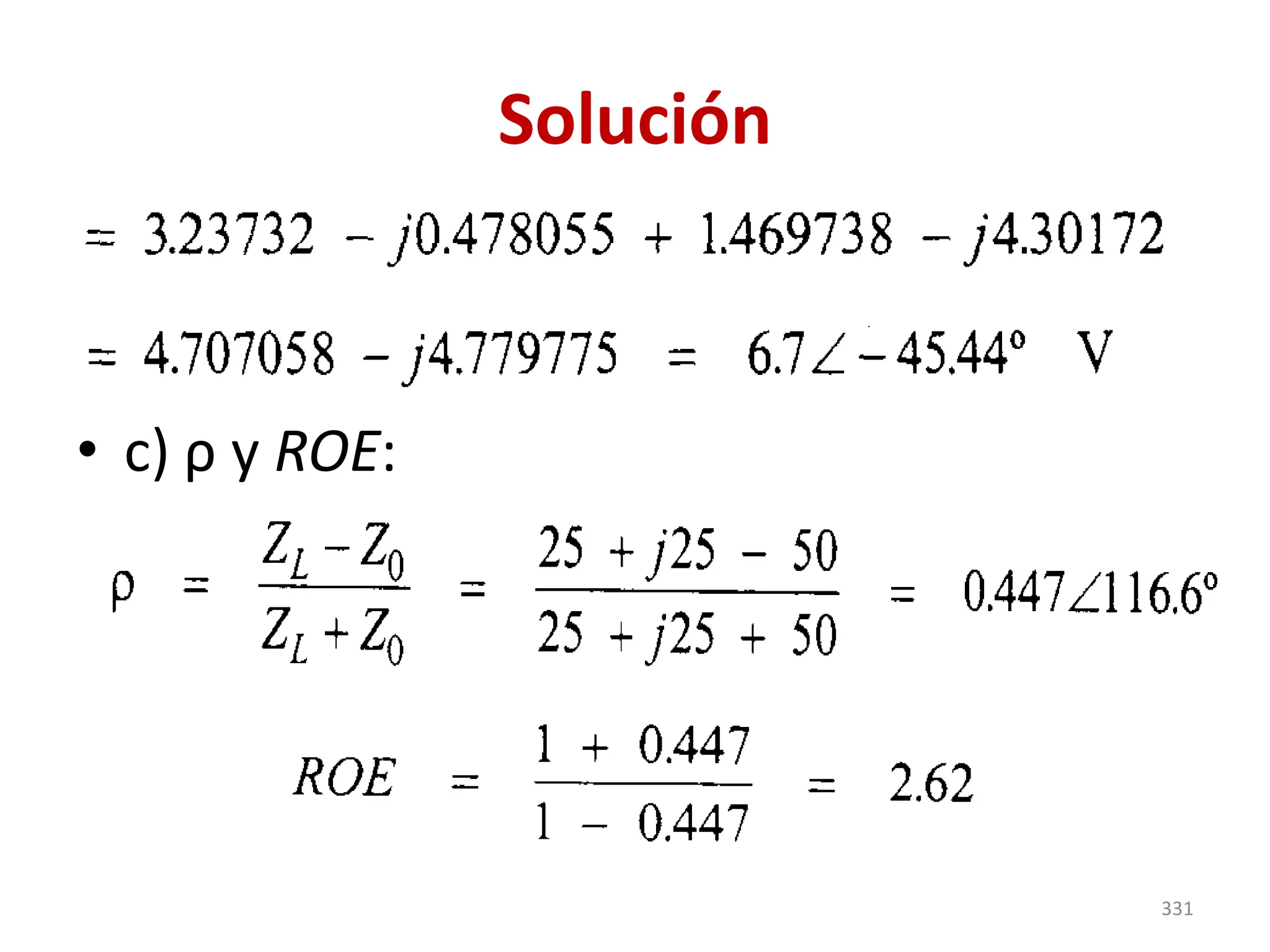
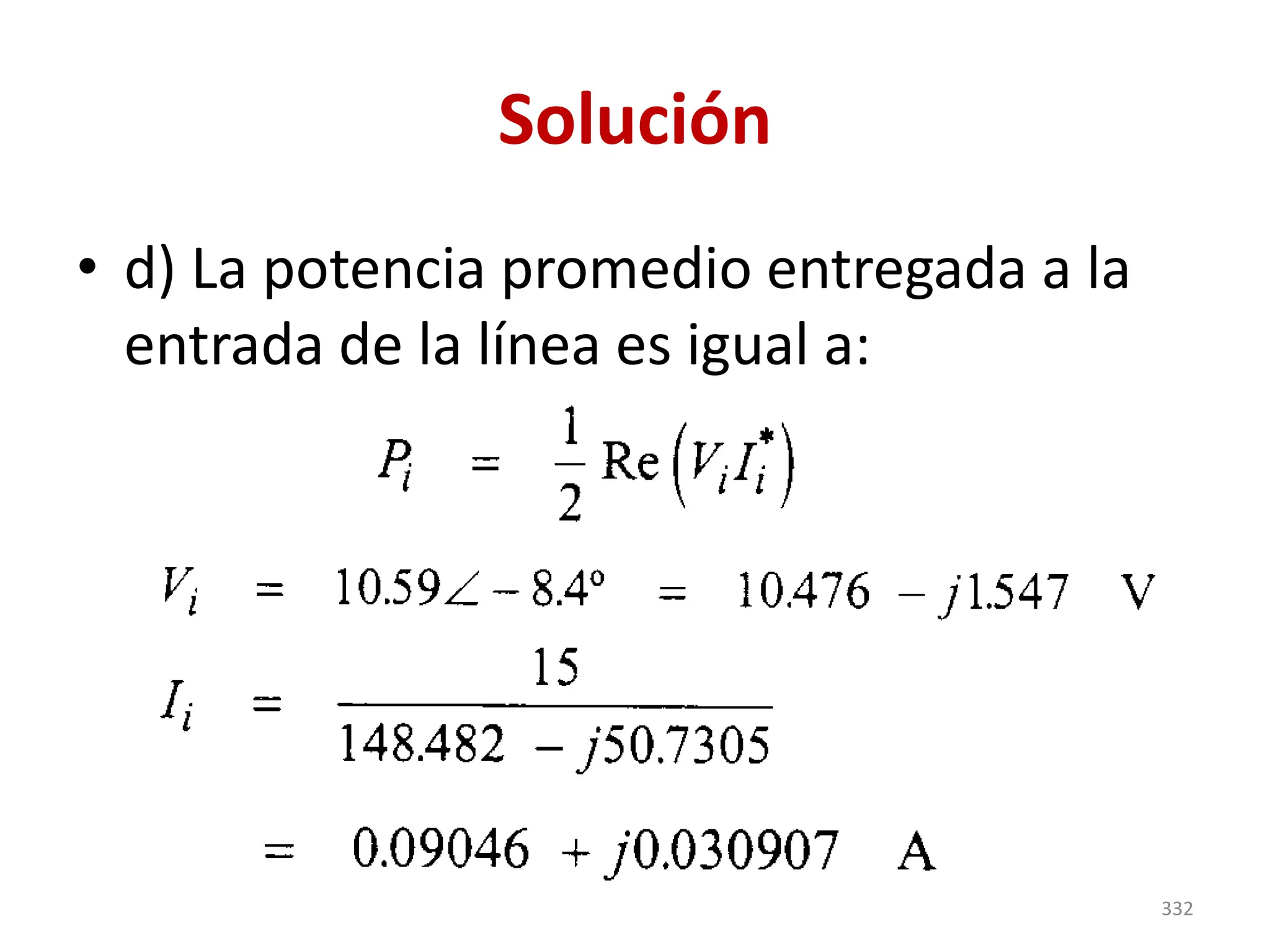
• a)el voltaje en la entrada de la línea, b)
el voltaje en la carga, c) la relación de
onda estacionaria, d) la potencia
promedio entregada a la entrada de la
línea, y e) la potencia promedio
entregada a la carga.
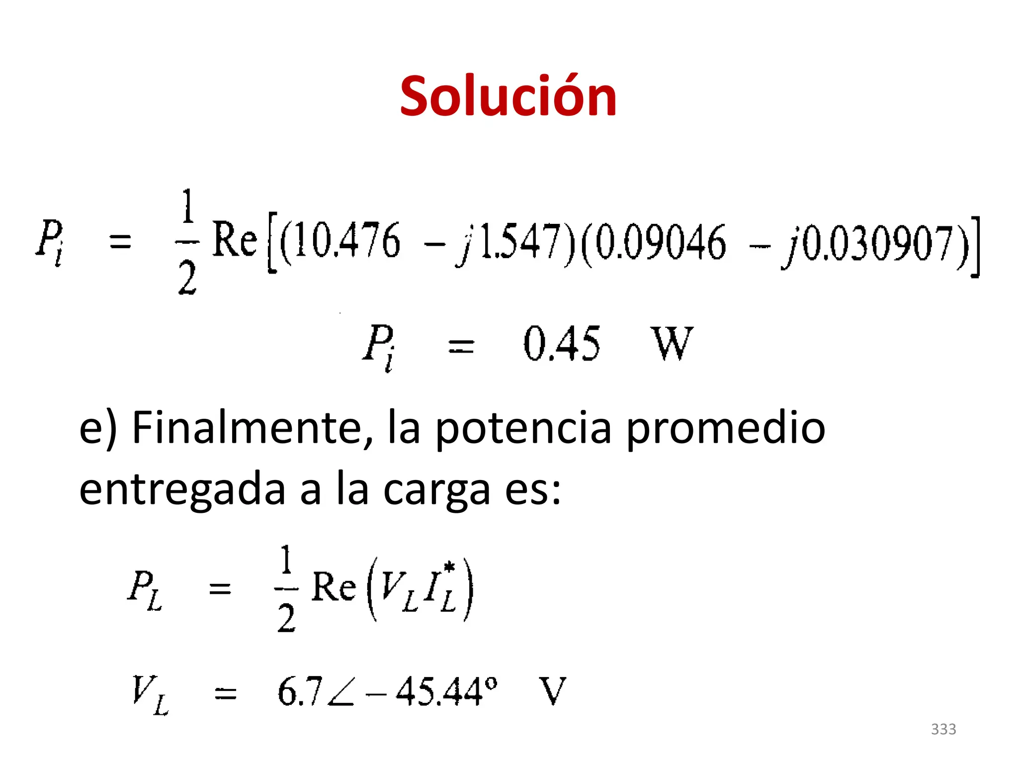
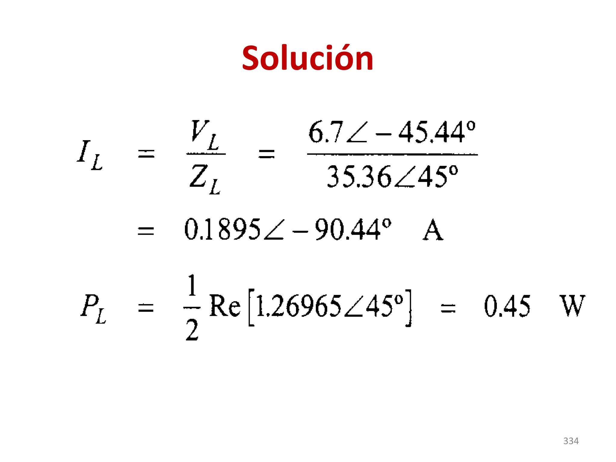
326
Solución
• La potenciainicial es igual a la potencia
entregada a la carga.
• Esto se obtiene aplicando el principio de
conservación de energía, ya que se
consideró que no hay pérdidas en la
línea.
• Esa potencia no es la máxima posible
porque la línea no está acoplada con la
carga.
335
336.
Solución
• Para obtenerla máxima potencia posible,
se necesitaría que ZL = 50 Ω. Bajo esta
condición, Zi sería también igual a 50 Ω y
Vi = 7.5/0° V e Ii = 0.15 /0° A.
• Por lo tanto, la potencia máxima de
entrada sería 0.5625 W, y para una línea
sin pérdidas esta potencia sería la misma
entregada en la carga.
336
337.
Solución
• En lapráctica las líneas sí tienen
pérdidas.
• De otra manera no habría que utilizar
repetidores en líneas muy largas.
• La atenuación se puede incorporar en la
solución de un problema, utilizando las
ecuaciones generales con γ = α + jβ.
337

![Suggested exercise
• An internal telephone line used to connect the
phone box to the outside network, consists of
two parallel copper conductors with a
diameter of 0.60 mm. The separation between
the conductor centers is 2.5 mm and the
insulating material between the two is
polyethylene. Calculate the L, C, R, and G
parameters per unit length at a frequency of 3
kHz.
[L = 942nH/m, C = 30 pF/m, R = 122 mΩ/m, G = 112 pƱ/m].
65](https://image.slidesharecdn.com/2-two-wirelinestheory-parta-250925234612-425ce6f2/75/2-Two-wire-lines-theory-Part-A-de-la-teoria-de-trasmision-de-dos-lineas-pdf-65-2048.jpg)
![Solution
• Thus, for example, for the specific point
where the load is, instantaneous
expressions are obtained by substituting
z = 6 m into the above equations.
• As regards the average power delivered
to the load, this must be equal to the
average input power, [considering
lossless line (α = 0)].
151](https://image.slidesharecdn.com/2-two-wirelinestheory-parta-250925234612-425ce6f2/75/2-Two-wire-lines-theory-Part-A-de-la-teoria-de-trasmision-de-dos-lineas-pdf-151-2048.jpg)
![Ejercicio 2.18.9 (Libro)
• Calculate the impedance seen at the
following points on the line: a) at the load, b)
at 10 cm before the load, c) at λ/4 before the
load, d) at λ/2 before the load, and e) at 3λ/2
before the load. [Z = 100 Ω, Z = 58.8 + j10.2
Ω, Z = 56.25 Ω, Z = 100 Ω, Z = 100 Ω].[Z = 100
Ω, Z = 58.8 + j10.2 Ω, Z = 56.25 Ω, Z = 100 Ω,
Z = 100 Ω].
175](https://image.slidesharecdn.com/2-two-wirelinestheory-parta-250925234612-425ce6f2/75/2-Two-wire-lines-theory-Part-A-de-la-teoria-de-trasmision-de-dos-lineas-pdf-175-2048.jpg)