Download as PDF, PPTX


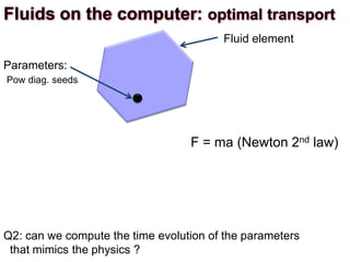
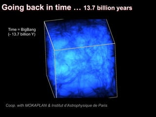
![Theorem: (direct consequence of MK duality, Brenier thm
alternative proof in [Aurenhammer, Hoffmann, Aronov 98] ):
Given a point set, there exists a unique weight vector W = [ψ(y1) ψ(y2) … ψ(ym)]
such that the Laguerre cells have the prescribed areas.
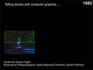
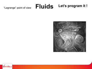
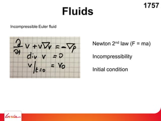
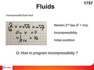
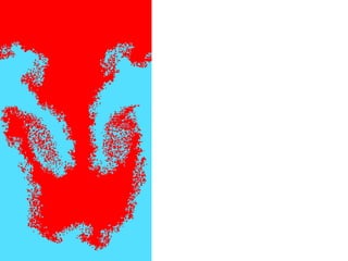
Fluids on the computer:
optimal transport](https://image.slidesharecdn.com/cgi2018-180707133434/85/CGI2018-keynote-fluids-simulation-87-320.jpg)
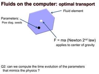
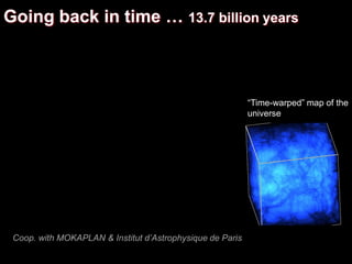
![Proof: G(ψ) =∑j ∫Lag ψ(yj) || x – yj ||2 - ψ(yj) dμ + ∑j ψ(yj) vj
Is a concave function of the weight vector [ψ(y1) ψ(y2) … ψ(ym)]
Theorem: (direct consequence of MK duality, Brenier thm
alternative proof in [Aurenhammer, Hoffmann, Aronov 98] ):
Given a point set, there exists a unique weight vector W = [ψ(y1) ψ(y2) … ψ(ym)]
such that the Laguerre cells have the prescribed areas.
Fluids on the computer:
optimal transport](https://image.slidesharecdn.com/cgi2018-180707133434/85/CGI2018-keynote-fluids-simulation-88-320.jpg)
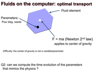
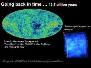
![Proof: G(ψ) =∑j ∫Lag ψ(yj) || x – yj ||2 - ψ(yj) dμ + ∑j ψ(yj) vj
Is a concave function of the weight vector [ψ(y1) ψ(y2) … ψ(ym)]
Theorem: (direct consequence of MK duality, Brenier thm
alternative proof in [Aurenhammer, Hoffmann, Aronov 98] ):
Given a point set, there exists a unique weight vector W = [ψ(y1) ψ(y2) … ψ(ym)]
such that the Laguerre cells have the prescribed areas.
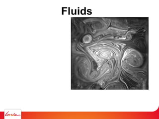
Fluids on the computer:
optimal transport](https://image.slidesharecdn.com/cgi2018-180707133434/85/CGI2018-keynote-fluids-simulation-89-320.jpg)
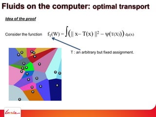
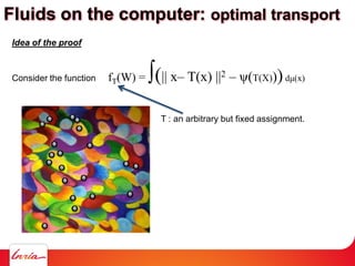
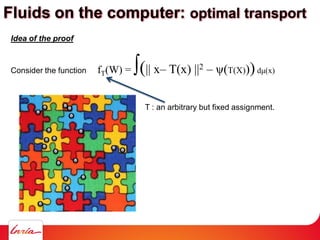
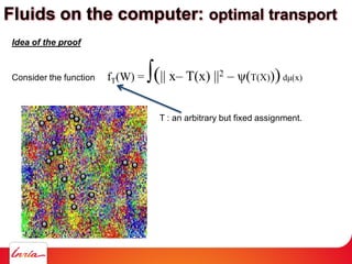
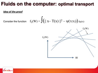
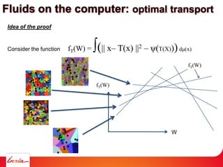
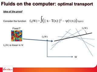
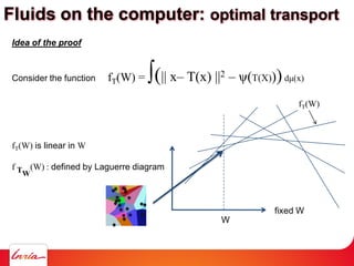
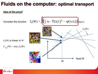
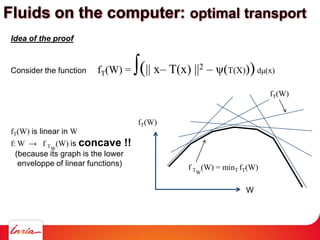
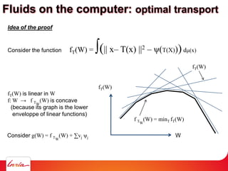
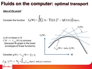
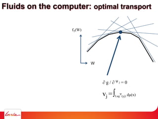
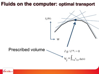
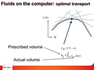
![Idea of the proof
Consider the function fT(W) = ∫(|| x– T(x) ||2 – ψ(T(X)))dμ(x)
The (unknown) weights W = [ψ(y1) ψ(y2) … ψ(ym)]
Fluids on the computer: optimal transport](https://image.slidesharecdn.com/cgi2018-180707133434/85/CGI2018-keynote-fluids-simulation-90-320.jpg)


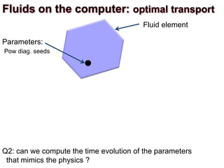
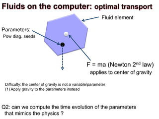
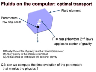
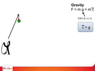
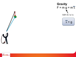
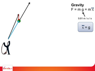
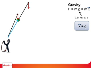
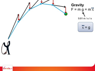
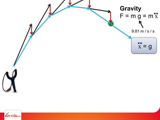
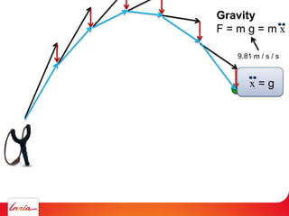
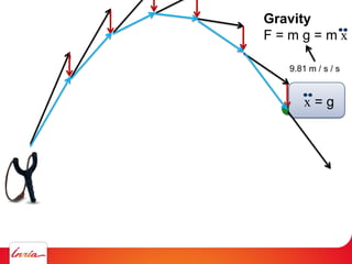
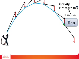
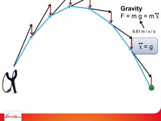
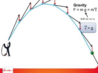
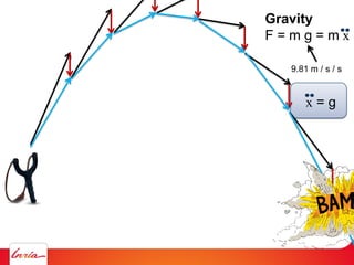
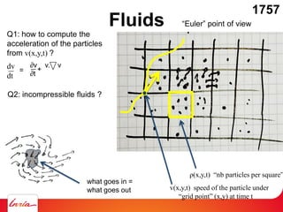
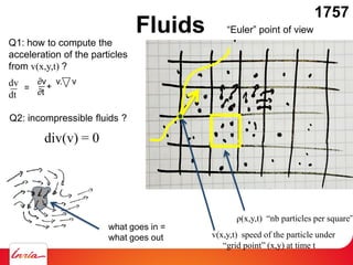
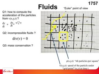
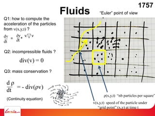
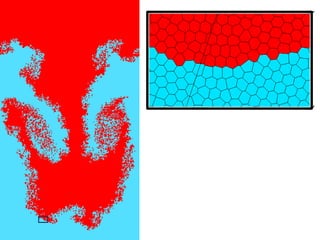
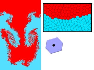
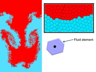
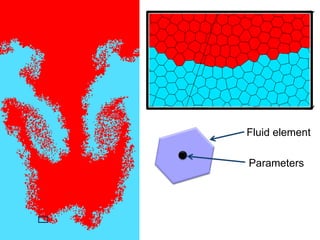
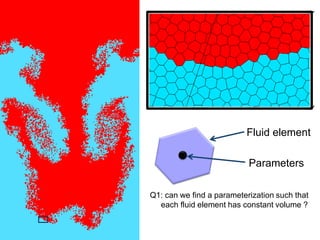
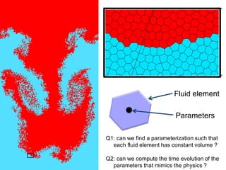
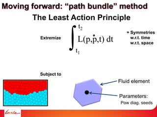
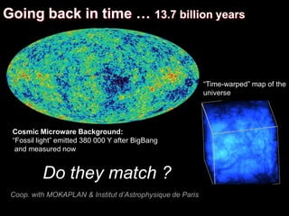
![Fluid element
Q2: can we compute the time evolution of the parameters
that mimics the physics ?
Parameters:
Pow diag. seeds
Fluids on the computer: optimal transport
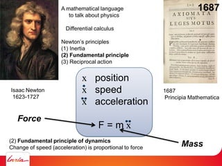
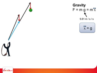
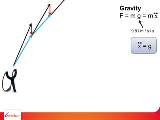
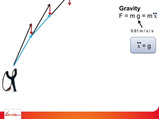
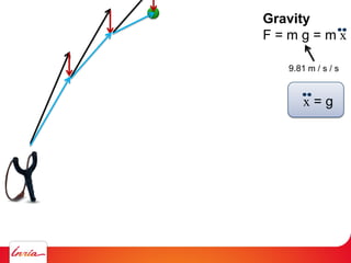
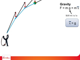
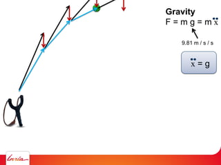
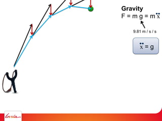
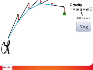
F = ma (Newton 2nd law)
applies to center of gravity
Difficulty: the center of gravity is not a variable/parameter
(1) Apply gravity to the parameters instead
(2) Add a spring so that it pulls the center of gravity
[Gallout Mérigot]
Converges to sol. of Euler](https://image.slidesharecdn.com/cgi2018-180707133434/85/CGI2018-keynote-fluids-simulation-114-320.jpg)


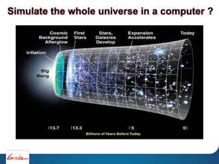
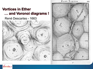
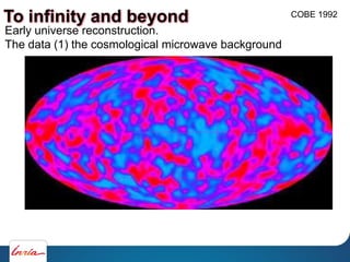
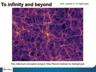

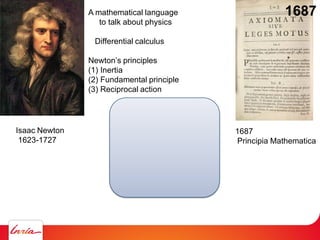
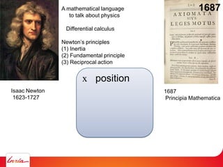
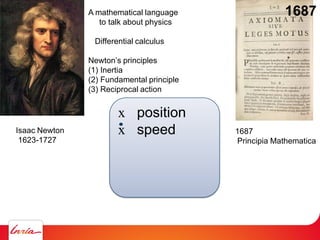
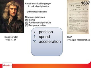
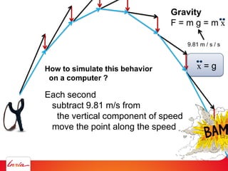
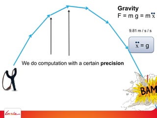
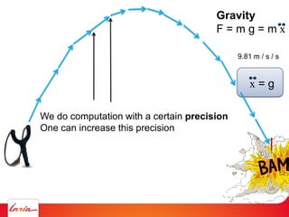
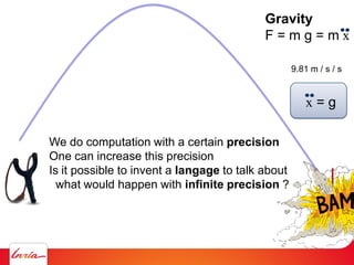
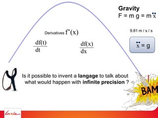
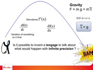
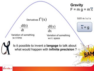
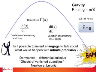
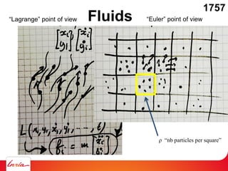
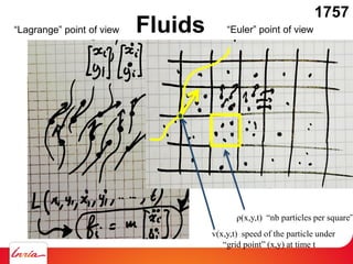
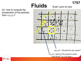
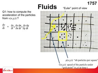
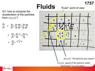
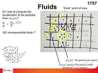
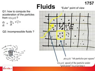
The document outlines various computational methods for simulating physics and fluids in computer graphics, discussing the mathematical principles underpinning these simulations, such as Newton's laws and fluid dynamics. It addresses the implementation of algorithms for optimal transport and the challenges of achieving precision in simulations. Key concepts include differential calculus, particle systems, and the use of diagrams such as Voronoi for modeling fluid behavior.