This document provides an introduction to computational finance using MATLAB. It discusses MATLAB basics like matrices, vectors, solving linear equations, and generating random numbers. Key points covered include: - MATLAB is well-suited for numerical linear algebra operations on matrices and vectors. - Functions like rand and randn are used to generate uniformly distributed and Gaussian/normal distributed random numbers, which are important in finance. - Histograms can be used to visualize the distributions of random numbers and converge to the probability density function as the number of samples increases.

1. Computational Finance using MATLAB
Brad Baxter
Department of Economics, Mathematics and Statistics,
Birkbeck College, University of London,
Malet Street, London WC1E 7HX
b.baxter@bbk.ac.uk
This is a short introduction to scientific computation in MATLAB. It is
designed for self-study by both GDFE and MSc students. 1
1. Introduction
These notes can be obtained from
http://econ109.econ.bbk.ac.uk/brad/CTFE/
and you can download lots of relevant material for MSc Financial Engineering
from
http://econ109.econ.bbk.ac.uk/brad/Methods/
This folder contains the current versions of methods notes.pdf and nabook.pdf.
The book Numerical Methods in Finance and Economics: A MATLAB-
based Introduction, by P. Brandimarte, contains many excellent examples,
and is strongly recommended for both CTFE and MSc Financial Engineering.
I also recommend the undergraduate-level textbook An Introduction to Financial
Option Valuation, by D. Higham, which is particularly suitable for CTFE.
All of the programs in this note also work with Octave, which is a free
quasi-clone of MATLAB, and can be found here:
http://www.gnu.org/software/octave/
Another good quasi-clone is
http://freemat.sourceforge.net/
You’re welcome to use the Computer Room; the door code is 5858.
1
Version: 201310241641

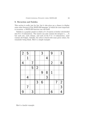
2. 2 Brad Baxter
2. MATLAB Basics
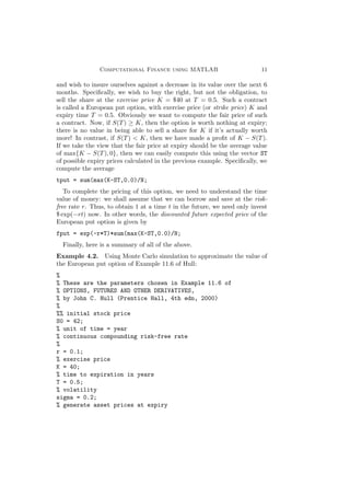
2.1. Matrices and Vectors
MATLAB (i.e. MATrix LABoratory) was designed for numerical linear
algebra.
Notation: a p × q matrix has p rows and q columns; its entries are usually
real numbers in these notes, but they can also be complex numbers. A p×1
matrix is also called a column vector, and a 1 × q matrix is called a row
vector. If p = q = 1, then it’s called a scalar.
We can easily enter matrices:
A = [1 2 3; 4 5 6; 7 8 9; 10 11 12]
In this example, the semi-colon tells Matlab the row is complete.
The transpose AT of a matrix A is formed by swapping the rows and
columns:
A = [1 2 3; 4 5 6; 7 8 9; 10 11 12]
AT = A’
Sometimes we don’t want to see intermediate results. If we add a semi-
colon to the end of the line, the MATLAB computes silently:
A = [1 2 3; 4 5 6; 7 8 9; 10 11 12];
AT = A’
Matrix multiplication is also easy. In this example, we compute AAT and
AT A.
A = [1 2 3; 4 5 6; 7 8 9; 10 11 12]
AT = A’
M1 = A*AT
M2 = AT*A
In general, matrix multiplication is non-commutative, as seen in Example
2.1.
Example 2.1. As another example, let’s take two column vectors u and
v in R4 and compute the matrix products u v and uv . The result might
surprise you at first glance.
u = [1; 2; 3; 4]
v = [5; 6; 7; 8]
u’*v
u*v’
Exercise 2.1. What’s the general formula for uv ?

3. Computational Finance using MATLAB 3
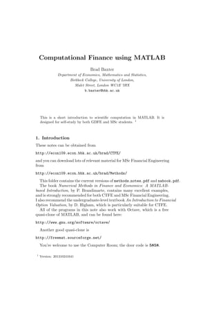
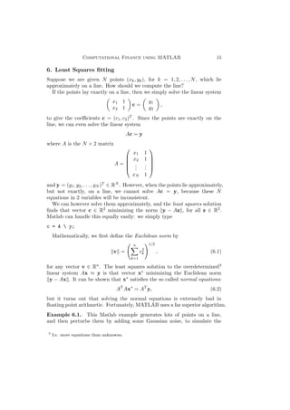
2.2. The sum function
It’s often very useful to be able to sum all of the elements in a vector, which
is very easy in Matlab:
u = [1 2 3 4]
sum(u)
The sum is also useful when dealing with matrices:
A = [1 2; 3 4]
sum(A)
You will see that Matlab has summed each column of the matrix.
2.3. Solving Linear Equations
MATLAB can also solve linear equations painlessly:
n = 10
% M is a random n x n matrix
M = randn(n);
% y is a random n x 1 matrix, or column vector.
y = randn(n,1);
% solve M x = y
x = My
% check the solution
y - M*x
We shall need to measure the length, or norm, of a vector, and this is
defined by
v = v2
1 + v2
2 + · · · + v2
n,
where v1, . . . , vn ∈ R are the components of the vector v; the corresponding
MATLAB function is norm(v). For example, to check the accuracy of the
numerical solution of Mx = y, we type norm(y - M*x).
It’s rarely necessary to compute the inverse M−1 of a matrix, because it’s
usually better to solve the corresponding linear system Mx = y using
x = My
as we did above. However, the corresponding MATLAB function is inv(M).
2.4. The MATLAB Colon Notation
MATLAB has a very useful Colon notation for generating lists of equally-
spaced numbers:
1:5

4. 4 Brad Baxter
will generate the integers 1, 2, . . . , 5, while
1:0.5:4
will generate 1, 1.5, 2, 2.5, . . . , 3.5, 4, i.e. the middle number is the step-size.
Example 2.2. This example illustrates a negative step-length and their
use to generate a vector.
v = [10:-1:1]’;
w = 2*v
We can easily extract parts of a matrix using the MATLAB colon notation.
A = [1 2 3; 4 5 6; 7 8 9; 10 11 12]
M = A(2:3, 2:3)
The following example illustrates the Matlab dot notation
Example 2.3. Consider the following MATLAB code.
A = [1 2; 3 4]
A^2
A.^2
The first command uses matrix multiplication to multiply A by itself, whilst
the second creates a new matrix by squaring every component of A.
Exercise 2.2. What does the following do?
sum([1:100].^2)
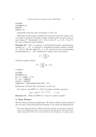
2.5. Graphics
Let’s learn more about graphics.
Example 2.4. Plotting a sine curve:
t = 0: pi/200: 2*pi;
y = sin(3*t);
plot(t,y)
Exercise 2.3. Replace plot(t,y) by plot(t,y,’o’) in the last example.
Example 2.5. See if you can predict the result of this code before typing
it:
t = 0: pi/200: 2*pi;
y = sin(3*t).^2;
plot(t,y)
Exercise 2.4. Use the plot function to plot the graph of the quadratic
p(x) = 2x2 − 5x + 2, for −3 ≤ x ≤ 3.

5. Computational Finance using MATLAB 5
Exercise 2.5. Use the plot function to plot the graph of the cubic q(x) =
x3 − 3x2 + 3x − 1, for −10 ≤ x ≤ 10.
Here’s a more substantial code fragment producing a cardioid as the
envelope of certain circles. You’ll also see this curve formed by light reflection
on the surface of tea or coffee if there’s a point source nearby (halogen bulbs
are good for this). It also introduces the axis command, which makes sure
that circles are displayed as proper circles (otherwise MATLAB rescales,
turning circles into ellipses).
Example 2.6. Generating a cardioid:
hold off
clf
t=0:pi/2000:2*pi;
plot(cos(t)+1,sin(t))
axis([-1 5 -3 3])
axis(’square’)
hold on
M=10;
for alpha=0:pi/M:2*pi
c=[cos(alpha)+1; sin(alpha)];
r = norm(c);
plot(c(1)+r*cos(t),c(2)+r*sin(t));
end
2.6. Getting help
You can type
help polar
to learn more about any particular command. Matlab has extensive documentation
built-in, and there’s lots of information available online.
3. Generating random numbers
Computers generate pseudorandom numbers, i.e. deterministic (entirely
predictable) sequences which mimic the statistical properties of random
numbers. Speaking informally, however, I shall often refer to “random
numbers” when, strictly speaking, “pseudorandom numbers” would be the
correct term. At a deeper level, one might question whether anything is truly
random, but these (unsolved) philosophical problems need not concern at
this stage.
We shall first introduce the extremely important rand and randn functions.

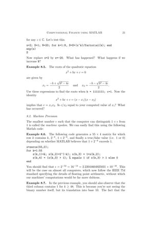
6. 6 Brad Baxter
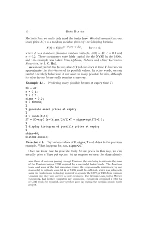
Despite their almost identical names, they are very different, as we shall
see, and should not be confused. The rand function generates uniformly
distributed numbers on the interval [0, 1], whilst the randn function generates
normally distributed, or Gaussian random numbers. In financial applications,
randn is extremely important.
Our first code generating random numbers can be typed in as a program,
using the create script facility, or just entered in the command window.
Example 3.1. Generating uniformly distributed random numbers:
N = 10000;
v=rand(N,1);
plot(v,’o’)
The function we have used here is rand(m,n), which produces an m × n
matrix of pseudorandom numbers, uniformly distributed in the interval [0, 1].
Using the plot command in these examples in not very satisfactory,
beyond convincing us that rand and randn both produce distributions of
points which look fairly random. For that reason, it’s much better to use a
histogram, which is introduced in the following example.
Example 3.2. Uniformly distributed random numbers and histograms:
N = 10000;
v=rand(N,1);
nbins = 20;
hist(v,nbins);
Here Matlab has divided the interval [0, 1] into 20 equal subintervals, i.e.
[0, 0.05], [0.05, 0.1], [0.1, 0.15], . . . , [0.90, 0.95], [0.95, 1],
and has simply drawn a bar chart: the height of the bar for the interval
[0, 0.05] is the number of elements of the vector v which lie in the interval
[0.0.05], and similarly for the other sub-intervals.
Exercise 3.1. Now experiment with this code: change N and nbins.
Example 3.3. Gaussian random numbers and histograms:
N = 100000;
v=randn(N,1);
nbins = 50;
hist(v,nbins);
Observe the obvious difference between this bell-shaped distribution and the
histogram for the uniform distribution.
Exercise 3.2. Now experiment with this code: change N and nbins. What
happens for large N and nbins?

7. Computational Finance using MATLAB 7
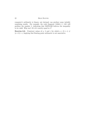
As we have seen, MATLAB can easily construct histograms for Gaussian
(i.e. normal) pseudorandom numbers. As N and nbins tend to infinity,
the histogram converges to a curve, which is called the probability density
function (PDF). The formula for this curve is
p(s) = (2π)−1/2
e−s2/2
, for s ∈ R,
and the crucial property of the PDF is
P(a < Z < b) =
b
a
p(s) ds.
Example 3.4. Good graphics is often fiddly, and this example uses some
more advanced features of MATLAB graphics commands to display the
histogram converging nicely to the PDF for the Gaussian. I will not explain
these fiddly details in the lecture, but you will learn much from further study
using the help facility. This example is more substantial so create a script,
i.e. a MATLAB program – I will explain this during the lecture. Every
line beginning with % is a comment. i.e. it is only there for the human
reader, not the computer. You will find comments extremely useful in your
programs.
% We generate a 1 x 5000 array of N(0,1) numbers
a = randn(1,5000);
% histogram from -3 to 3 using bins of size .2
[n,x] = hist(a, [-3:.2:3]);
% draw a normalized bar chart of this histogram
bar(x,n/(5000*.2));
% draw the next curve on the same plot
hold on
% draw the Gaussian probability density function
plot(x, exp(-x.^2/2)/sqrt(2*pi))
%
% Note the MATLAB syntax here: x.^2 generates a new array
% whose elements are the squares of the original array x.
hold off
Exercise 3.3. Now repeat this experiment several times to get a feel for
how the histogram matches the density for the standard normal distribution.
Replace the magic numbers 5000 and 0.2 by N and Delta and see for yourself
how much it helps or hinders to take more samples or smaller size bins.
3.1. The Central Limit Theorem
Where does the Gaussian distribution come from? Why does it occur in
so many statistical applications? It turns out that averages of random

8. 8 Brad Baxter
variables are often well approximated by Gaussian random variables, if the
random variables are not too wild, and this important theorem is called
the Central Limit Theorem. The next example illustrates the Central Limit
Theorem, and shows that averages of independent, uniformly distributed
random variables converge to the Gaussian distribution.
Example 3.5. This program illustrates the Central Limit Theorem: suitably
scaled averages of uniformly distributed random variables look Gaussian, or
normally distributed. First we create a 20 × 10000 matrix of pseudorandom
numbers uniformly distributed on the interval [0, 1], using the rand functions.
We then sum every column of this matrix and divide by
√
20.
m = 20;
n = 10000;
v = rand(m,n);
%
% We now sum each column of this matrix, divide by sqrt(m)
% and histogram the new sequence
%
nbins = 20
w = sum(v)/sqrt(m);
hist(w,nbins);
Exercise 3.4. Play with the constants m and n in the last example.
3.2. Gaussian Details
The Matlab randn command generates Gaussian pseudorandom numbers
with mean zero and variance one; we write this N(0, 1), and such random
variables are said to be normalized Gaussian, or standard normal. If Z
is a normalized Gaussian random variable, then the standard notation to
indicate this is Z ∼ N(0, 1), where “∼” means “is distributed as”. We can
easily demonstrate these properties in Matlab:
Example 3.6. Here we generate n normalized Gaussian pseudorandom
numbers Z1, . . . , Zn, and then calculate their sample mean
µ =
1
n
n
k=1
Zk
and their sample variance
σ2
=
1
n
n
k=1
Z2
k,
as follows.

9. Computational Finance using MATLAB 9
n=10000;
Z=randn(n,1);
mean(Z)
mean(Z.^2)
Experiment with this code, increasing n to 106, say.
Obviously not all random variables have mean zero and unit variance, but
it’s simple to generate Gaussian random variables with any given mean µ
and variance σ2. Specifically, if Z ∼ N(0, 1), then W = µ + σZ ∼ N(µ, σ2).
It’s easy to illustrate this in Matlab.
Example 3.7. Here we generate n normalized Gaussian pseudorandom
numbers Z1, . . . , Zn, to represent a normalized Gaussian random variable
Z ∼ N(0, 1). We then define W = µ + σZ, and generate the corresponding
pseudorandom W1, . . . , Wn, finding their sample mean and variance
µ =
1
n
n
k=1
Zk
and their sample variance
σ2
=
1
n
n
k=1
(Zk − µ)2
,
as follows.
n=10000;
Z=randn(n,1);
mu = 1; sigma = 0.2;
W = mu + sigma*Z;
mu_hat = mean(W)
sigma_hat = sqrt(mean((W-mu_hat).^2))
Experiment with this code, increasing n to 106, say.
For reference, the PDF for a N(0, σ2) random variable is given by
p(s) = (2πσ2
)−1/2
e−s2/(2σ2)
, s ∈ R.
Exercise 3.5. What the PDF for a N(µ, σ2) random variable?
4. Some Finance
Now let’s discuss a financial application. We shall use Monte Carlo simulation.2
You can find a full mathematical treatment in my notes for Mathematical
2
This name originated with the brilliant mathematician John von Neumann, during his
work on the Manhattan Project, the secret project building the first American atomic
bombs during World War II. In the first Monte Carlo simulation, the sample paths

10. 10 Brad Baxter
Methods, but we really only need the basics here. We shall assume that our
share price S(t) is a random variable given by the following formula
S(t) = S(0)e(r−σ2/2)t+σ
√
tZ
, for t > 0,
where Z is a standard Gaussian random variable, S(0) = 42, r = 0.1 and
σ = 0.2. These parameters were fairly typical for the NYSE in the 1990s,
and this example was taken from Options, Futures and Other Derivative
Securities, by J. C. Hull.
We cannot predict the future price S(T) of our stock at time T, but we can
approximate the distribution of its possible values. In other words, we can
predict the likely behaviour of our asset in many possible futures, although
its value in our future sadly remains a mystery.
Example 4.1. Predicting many possible futures at expiry time T:
S0 = 42;
r = 0.1;
T = 0.5;
sigma = 0.2;
N = 100000;
%
% generate asset prices at expiry
%
Z = randn(N,1);
ST = S0*exp( (r-(sigma^2)/2)*T + sigma*sqrt(T)*Z );
%
% display histogram of possible prices at expiry
%
nbins=40;
hist(ST,nbins);
Exercise 4.1. Try various values of N, sigma, T and nbins in the previous
example. What happens for, say, sigma=20?
Once we know how to generate likely future prices in this way, we can
actually price a Euro put option: let us suppose we own the share already
were those of neutrons passing through Uranium, the aim being to estimate the mass
of the Uranium isotope U235 required for a successful fission bomb. The American
team used some of the first computers (more like programmable calculators, by our
standards) to estimate some 64 kg of U235 would be sufficient, which was achievable
using the cumbersome technology required to separate the 0.07% of U235 from common
Uranium ore; they were correct in their estimates. The German team, led by Werner
Heisenberg, had neither computers nor simulation. Heisenberg estimated a 1000 kg
of U235 would be required, and therefore gave up, ending the German atomic bomb
project.

11. Computational Finance using MATLAB 11
and wish to insure ourselves against a decrease in its value over the next 6
months. Specifically, we wish to buy the right, but not the obligation, to
sell the share at the exercise price K = $40 at T = 0.5. Such a contract
is called a European put option, with exercise price (or strike price) K and
expiry time T = 0.5. Obviously we want to compute the fair price of such
a contract. Now, if S(T) ≥ K, then the option is worth nothing at expiry;
there is no value in being able to sell a share for K if it’s actually worth
more! In contrast, if S(T) < K, then we have made a profit of K − S(T).
If we take the view that the fair price at expiry should be the average value
of max{K − S(T), 0}, then we can easily compute this using the vector ST
of possible expiry prices calculated in the previous example. Specifically, we
compute the average
tput = sum(max(K-ST,0.0)/N;
To complete the pricing of this option, we need to understand the time
value of money: we shall assume that we can borrow and save at the risk-
free rate r. Thus, to obtain 1 at a time t in the future, we need only invest
$ exp(−rt) now. In other words, the discounted future expected price of the
European put option is given by
fput = exp(-r*T)*sum(max(K-ST,0.0)/N;
Finally, here is a summary of all of the above.
Example 4.2. Using Monte Carlo simulation to approximate the value of
the European put option of Example 11.6 of Hull:
%
% These are the parameters chosen in Example 11.6 of
% OPTIONS, FUTURES AND OTHER DERIVATIVES,
% by John C. Hull (Prentice Hall, 4th edn, 2000)
%
%% initial stock price
S0 = 42;
% unit of time = year
% continuous compounding risk-free rate
%
r = 0.1;
% exercise price
K = 40;
% time to expiration in years
T = 0.5;
% volatility
sigma = 0.2;
% generate asset prices at expiry

12. 12 Brad Baxter
N=10000;
Z = randn(N,1);
ST = S0*exp( (r-(sigma^2)/2)*T + sigma*sqrt(T)*Z );
% calculate put contract values at expiry
fput = max(K - ST,0.0);
% average put values at expiry and discount to present
mc_put = exp(-r*T)*sum(fput)/N
Exercise 4.2. Modify this example to calculate the Monte Carlo approximation
for a European call, for which the contract value at expiry is given by
max(ST - K, 0)
Exercise 4.3. Modify the code to calculate the Monte Carlo approximation
to a digital call, for which the contract value at expiry is given by
(ST > K);
5. Brownian Motion
The mathematics of Brownian motion is covered in my Mathematical Methods
lectures, during the first term of MSc Financial Engineering. However, it
is possible to obtain a good feel for Brownian motion using some simple
MATLAB examples.
Our next example generates discrete Brownian motion, as well as introducing
some more MATLAB language tools. Mathematically, we’re generating a
random function W : [0, ∞) → R using the equation
W(kh) =
√
h (Z1 + Z2 + · · · + Zk) , for k = 1, 2, . . . ,
where h > 0 is a positive time step and Z1, Z2, . . . , Zk are independent
N(0, 1) random variables.
Example 5.1. One basic way to generate Brownian motion:
T = 1; N = 500; dt = T/N;
dW = zeros(1,N);
W = zeros(1,N);
dW(1) = sqrt(dt)*randn;
W(1) = dW(1);
for j = 2:N
dW(j) = sqrt(dt)*randn;
W(j) = W(j-1) + dW(j);
end
plot([0:dt:T],[0,W])

13. Computational Finance using MATLAB 13
The MATLAB function cumsum calculates the cumulative sum performed
by the for loop in the last program, which makes life much easier.
Example 5.2. A more concise way to generate Brownian motion:
T = 1; N = 10000; dt = T/N;
dW = sqrt(dt)*randn(1,N); plot([0:dt:T],[0,cumsum(dW)])
Now play with this code, changing T and N.
Example 5.3. We can also use cumsum to generate many Brownian sample
paths:
T = 1; N = 500; dt = T/N;
nsamples = 10;
hold on
for k=1:nsamples
dW = sqrt(dt)*randn(1,N); plot([0:dt:T],[0,cumsum(dW)])
end
Exercise 5.1. Increase nsamples in the last example. What do you see?
5.1. Geometric Brownian Motion (GBM)
The idea that it can be useful to model asset prices using random functions
was both surprising and implausible when Louis Bachelier first suggested
Brownian motion in his thesis in 1900. There is an excellent translation of
his pioneering work in Louis Bachelier’s Theory of Speculation: The Origins
of Modern Finance, by M. Davis and A. Etheridge. However, as you have
already seen, a Brownian motion can be both positive and negative, whilst a
share price can only be positive, so Brownian motion isn’t quite suitable as a
mathematical model for share prices. Its modern replacement is to take the
exponential, and the result is called Geometric Brownian Motion (GBM).
In other words, the most common mathematical model in modern finance is
given by
S(t) = S(0)eµt+σW(t)
, for t > 0,
where µ ∈ R is called the drift and σ is called the volatility.
Example 5.4. Generating GBM:
T = 1; N = 500; dt = T/N;
t = 0:dt:T;
dW = sqrt(dt)*randn(1,N);
mu = 0.1; sigma = 0.01;
plot(t,exp(mu*t + sigma*[0,cumsum(dW)]))

14. 14 Brad Baxter
Exercise 5.2. Now experiment by increasing and decreasing the volatility
sigma.
In mathematical finance, we cannot predict the future, but we estimate
general future behaviour, albeit approximately. For this we need to generate
several Brownian motion sample paths, i.e. several possible futures for our
share. The key command will be randn(M,N), which generates an M × N
matrix of independent Gaussian random numbers, all of which are N(0, 1).
We now need to tell the cumsum function to cumulatively sum along each
row, and this is slightly more tricky.
Example 5.5. Generating several GBM sample paths:
T = 1; N = 500; dt = T/N;
t = 0:dt:T;
M=10;
dW = sqrt(dt)*randn(M,N);
mu = 0.1; sigma = 0.01;
S = exp(mu*ones(M,1)*t + sigma*[zeros(M,1), cumsum(dW,2)]);
plot(t,S)
Here the MATLAB function ones(p,q) creates a p × q matrix of ones,
whilst zeros(p,q) creates a p × q matrix of zeros. The matrix product
ones(M,1)*t is a simple way to create an M × N matrix whose every row
is a copy of t.
Exercise 5.3. Experiment with various values of the drift and volatility.
Exercise 5.4. Copy the use of the cumsum function in Example 5.5 to
avoid the for loop in Example 5.3.

15. Computational Finance using MATLAB 15
6. Least Squares fitting
Suppose we are given N points (xk, yk), for k = 1, 2, . . . , N, which lie
approximately on a line. How should we compute the line?
If the points lay exactly on a line, then we simply solve the linear system
x1 1
x2 1
c =
y1
y2
,
to give the coefficients c = (c1, c2)T . Since the points are exactly on the
line, we can even solve the linear system
Ac = y
where A is the N × 2 matrix
A =





x1 1
x2 1
...
...
xN 1





and y = (y1, y2, . . . , yN )T ∈ RN . However, when the points lie approximately,
but not exactly, on a line, we cannot solve Ac = y, because these N
equations in 2 variables will be inconsistent.
We can however solve them approximately, and the least squares solution
finds that vector c ∈ R2 minimizing the norm y − Az , for all z ∈ R2.
Matlab can handle this equally easily: we simply type
c = A y;
Mathematically, we first define the Euclidean norm by
v =
n
k=1
v2
k
1/2
, (6.1)
for any vector v ∈ Rn. The least squares solution to the overdetermined3
linear system Ax ≈ y is that vector x∗ minimizing the Euclidean norm
y − Ax . It can be shown that x∗ satisfies the so called normal equations:
AT
Ax∗
= AT
y, (6.2)
but it turns out that solving the normal equations is extremely bad in
floating point arithmetic. Fortunately, MATLAB uses a far superior algorithm.
Example 6.1. This Matlab example generates lots of points on a line,
and then perturbs them by adding some Gaussian noise, to simulate the
3
I.e. more equations than unknowns.

16. 16 Brad Baxter
imperfections of real data. It then computes the least squares line of best
fit.
%
% We first generate some
% points on a line and add some noise
%
a0=1; b0=0;
n=100; sigma=0.1;
x=randn(n,1);
y=a0*x + b0 + sigma*randn(n,1);
%
% Here’s the least squares linear fit
% to our simulated noisy data
%
A=[x ones(n,1)];
c = Ay;
%
% Now we plot the points and the fitted line.
%
plot(x,y,’o’);
hold on
xx = -2.5:.01:2.5;
yy=a0*xx+b0;
zz=c(1)*xx+c(2);
plot(xx,yy,’r’)
plot(xx,zz,’b’)
Exercise 6.1. What happens when we increase the parameter sigma?
Exercise 6.2. Least Squares fitting is an extremely useful technique, but
it is extremely sensitive to outliers. Here is a MATLAB code fragment to
illustrate this:
%
% Now let’s massively perturb one data value.
%
y(n/2)=100;
cnew=Ay;
%
% Exercise: display the new fitted line. What happens when we vary the
% value and location of the outlier?
%

17. Computational Finance using MATLAB 17
7. General Least Squares
There is no reason to restrict ourselves to linear fits. If we wanted to fit
a quadratic p(x) = p0 + p1x + p2x2 to the data (x1, y1), . . . , (xN , yN ), then
we can still compute the least squares solution to the overdetermined linear
system
Ap ≈ y,
where p = (p0, p1, p2)T ∈ R3 and A is now the N × 3 matrix given by
A =





x2
1 x1 1
x2
2 x2 1
...
...
...
x2
N xN 1





.
This requires a minor modification to Example 6.1.
Example 7.1. Generalizing Example 6.1, we generate a quadratic, perturb
the quadratic by adding some Gaussian noise, and then fit a quadratic to
the noisy data.
%
% We first generate some
% points using the quadratic x^2 - 2x + 1 and add some noise
%
a0=1; b0=-2; c0=1;
n=100; sigma=0.1;
x=randn(n,1);
y=a0*(x.^2) + b0*x + c0 + sigma*randn(n,1);
%
% Here’s the least squares quadratic fit
% to our simulated noisy data
%
A=[x.^2 x ones(n,1)];
c = Ay;
%
% Now we plot the points and the fitted quadratic
%
plot(x,y,’o’);
hold on
xx = -2.5:.01:2.5;
yy=a0*(xx.^2)+b0*xx + c0;
zz=c(1)*(xx.^2)+c(2)*xx + c(3);
plot(xx,yy,’r’)
plot(xx,zz,’b’)

18. 18 Brad Baxter
Exercise 7.1. Increase sigma in the previous example, as for Example 6.1.
Further, explore the effect of choosing a large negative outlier by adding the
line y(n/2)=-10000; before solving for c.
There is absolutely no need to restrict ourselves to polynomials. Suppose
we believe that our data (x1, y1), . . . , (xN , yN ) are best modelled by a function
of the form
s(x) = c0 exp(−x) + c1 exp(−2x) + c2 exp(−3x).
We now compute the least squares solution to the overdetermined linear
system Ap ≈ y, where p = (p0, p1, p2)T ∈ R3 and
A =





e−x1 e−2∗x1 e−3x1
e−x2 e−2∗x2 e−3x2
...
...
...
e−xN e−2∗xN e−3xN





.
Example 7.2. %
% We first generate some
% points using the function
% a0*exp(-x) + b0*exp(-2*x) + c0*exp(-3*x)
% and add some noise
%
a0=1; b0=-2; c0=1;
n=100; sigma=0.1;
x=randn(n,1);
y=a0*exp(-x) + b0*exp(-2*x) + c0*exp(-3*x) + sigma*randn(n,1);
%
% Here’s the least squares fit
% to our simulated noisy data
%
A=[exp(-x) exp(-2*x) exp(-3*x)];
c = Ay;
%
% Now we plot the points and the fitted quadratic
%
plot(x,y,’o’);
hold on
xx = -2.5:.01:2.5;
yy=a0*exp(-xx)+b0*exp(-2*xx) + c0*exp(-3*xx);
zz=c(1)*exp(-xx)+c(2)*exp(-2*xx) + c(3)*exp(-3*xx);
plot(xx,yy,’r’)
plot(xx,zz,’b’)

19. Computational Finance using MATLAB 19
8. Warning Examples
In the 1960s, mainframe computers became much more widely available
in universities and industry, and it rapidly became obvious that it was
necessary to provide software libraries to solve common numerical problems,
such as the least squares solution of linear systems. This was a golden age for
the new discipline of Numerical Analysis, straddling the boundaries of pure
mathematics, applied mathematics and computer science. Universities and
national research centres provided this software, and three of the pioneering
groups were here in Britain: the National Physical Laboratory, in Teddington,
the Atomic Energy Research Establishment, near Oxford, and the Numerical
Algorithms Group (NAG), in Oxford. In the late 1980s, all of this code
was incorporated into MATLAB. The great advantage of this is that the
numerical methods chosen by MATLAB are excellent and extremely well
tested. However any method can be defeated by a sufficiently nasty problem,
so you should not become complacent. The following matrix is usually called
the Hilbert matrix, and seems quite harmless on first contact: it is the n × n
matrix H(n) whose elements are given by the simple formula
H
(n)
jk =
1
j + k + 1
, 1 ≤ j, k ≤ n.
MATLAB knows about the Hilbert matrix: you can generate the 20 × 20
Hilbert matrix using the command A = hilb(20);. The Hilbert matrix is
notoriously ill-conditioned, and the practical consequence of this property is
shown here:
Example 8.1. %
% A is the n x n Hilbert matrix
%
n = 15;
A = hilb(n);
%
%
%
v = [1:n]’;
w = A * v;
%
% If we now solve w = A*vnew using vnew = A w,
% then we should find that vnew is the vector v.
% Unfortunately this is NOT so . . .
%
vnew = A w
Exercise 8.1. Try increasing n in the previous example.

20. 20 Brad Baxter
8.1. Floating Point Warnings
Computers use floating point arithmetic. You shouldn’t worry about this
too much, because the relative error in any arithmetic operation is roughly
10−16, and we shall make this more precise below. However, it is not the same
as real arithmetic. In particular, errors can be greatly magnified and the
order of evaluation can affect results. For example, floating point addition
is commutative, but not associative: a + (b + c) = (a + b) + c, in general.
In this section, we want to see the full form of numbers, and not just the
first few decimal places. To do this, use the MATLAB command format
long.
Example 8.2. Prove that
1 − cos x
x2
=
sin2
x
x2 (1 + cos x)
.
Let’s check this identity in MATLAB:
for k=1:8, x=10^(-k); x^(-2)*(1-cos(x)), end
for k=1:8, x=10^(-k); x^(-2)*sin(x)^2/(1+cos(x)), end
Explain these calculations. Which is closer to the truth?
We can also avoid using loops using MATLAB’s dot notation for pointwise
operations. I have omitted colons in the next example to illustrate this:
x=10.^(-[1:8])
1-cos(x)
(sin(x).^2) ./ (1+cos(x))
Example 8.3. Prove that
√
x + 1 −
√
x =
1
√
x + 1 +
√
x
,
for x > 0. Now explain what happens when we try these algebraically equal
expressions in MATLAB:
x=123456789012345;
a=sqrt(x+1)-sqrt(x)
a = 4.65661287307739e-08
b=1/(sqrt(x+1) + sqrt(x))
b = 4.50000002025000e-08
Which is correct?
Example 8.4. You should know from calculus that
exp(z) =
∞
k=0
zk
k!
,

21. Computational Finance using MATLAB 21
for any z ∈ C. Let’s test this.
x=2; S=1; N=20; for k=1:N, S=S+(x^k)/factorial(k); end
exp(x)
S
Now replace x=2 by x=-20. What has happened? What happens if we
increase N?
Example 8.5. The roots of the quadratic equation
x2
+ bx + c = 0
are given by
x1 =
−b +
√
b2 − 4c
2
and x2 =
−b −
√
b2 − 4c
2
.
Use these expressions to find the roots when b = 1111111; c=1. Now the
identity
x2
+ bx + c = (x − x1)(x − x2)
implies that c = x1x2. Is c/x2 equal to your computed value of x1? What
has occurred?
8.2. Machine Precision
The smallest number such that the computer can distinguish 1 + from
1 is called the machine epsilon. We can easily find this using the following
Matlab code:
Example 8.6. The following code generates a 55 × 4 matrix for which
row k contains k, 2−k, 1 + 2−k, and finally a true/false value (i.e. 1 or 0)
depending on whether MATLAB believes that 1 + 2−k exceeds 1.
x=zeros(55,0);
for k=1:55
x(k,1)=k; x(k,2)=2^(-k); x(k,3) = 1+x(k,2);
x(k,4) = (x(k,3) > 1); % equals 1 if x(k,3) > 1 else 0
end
You should find that = 2−52 = 16−13 = 2.22044604925031 × 10−16. This
will be the case on almost all computers, which now follow the IEEE 754
standard specifying the details of floating point arithmetic, without which
our machines’ computations would be far more dubious.
Example 8.7. In the previous example, you should also observe that the
third column contains 1 for k ≥ 48. This is because you’re not seeing the
binary number itself, but its translation into base 10. The fact that the

22. 22 Brad Baxter
computer’s arithmetic is binary, not decimal, can produce some initially
surprising results. For example, the code fragment (10*0.1 < 10) will
produce the number 1, indicating that MATLAB believes the inequality
to be valid. Why isn’t 10 ∗ 0.1 exactly equal to 1?
Exercise 8.2. Construct values of a, b and c for which a + (b + c) =
(a + b) + c, implying that floating point arithmetic is not associative.

23. Computational Finance using MATLAB 23
9. Recursion and Sudoku
This section is really just for fun, but it also gives me a chance to display
some other features of the MATLAB language, of which the most important
is recursion: a MATLAB function can call itself.
Sudoku is a popular puzzle in which a 9 × 9 matrix is further sub-divided
into 9 3 × 3 submatrices. The matrix can only contain the integers 1, . . . , 9,
but each row, each column, and each of the 9 3 × 3 submatrices, must
contain all 9 digits. Initially, the solver is faced with some given values, the
remainder being blank. Here’s a simple example:
2 5 3 9 1
1 4
4 7 2 8
5 2
9 8 1
4 3
3 6 7 2
7 3
9 3 6 4
Here’s a harder example:

24. 24 Brad Baxter
2 3 9 7
1
4 7 2 8
5 2 9
1 8 7
4 3
6 7 1
7
9 3 2 6 5
It’s not too difficult to write a MATLAB program which can solve any
Sudoku. You can download a simple Sudoku solver (sud.m) from my office
machine:
http://econ109.econ.bbk.ac.uk/brad/CTFE/matlab_code/sudoku/
Here’s the MATLAB code for the solver:
function A = sud(A)
global cc
cc = cc+1;
% find all empty cells
[yy xx]=find(A==0);
if length(xx)==0
disp(’solution’)
disp(A);
return
end
x=xx(1);
y=yy(1);

25. Computational Finance using MATLAB 25
for i=1:9 % try 1 to 9
% compute the 3 x 3 block containing this element
y1=1+3*floor((y-1)/3); % find 3x3 block
x1=1+3*floor((x-1)/3);
% check if i is in this element’s row, column or 3 x 3 block
if ~( any(A(y,: )==i) | any(A(:,x)==i) | any(any(A(y1:y1+2,x1:x1+2)==i)) )
Atemp=A;
Atemp(y,x)=i;
% recursively call this function
Atemp=sud(Atemp);
if all(all(Atemp))
A=Atemp; % ... the solution
return; % and that’s it
end
end
end
Download and save this file as sud.m. You can try the solver with the
following example:
%
% Here’s the initial Sudoku; zeros indicate blanks.
%
M0 = [
0 4 0 0 0 0 0 6 8
7 0 0 0 0 5 3 0 0
0 0 9 0 2 0 0 0 0
3 0 0 5 0 0 0 0 7
0 0 1 2 6 4 9 0 0
2 0 0 0 0 7 0 0 6
0 0 0 0 5 0 7 0 0
0 0 6 3 0 0 0 0 1
4 8 0 0 0 0 0 3 0];
M0
M = M0;
%
% cc counts the number of calls to sud, so it one measure
% of Sudoku difficulty.
%
global cc = 0;
sud(M);
cc

26. 26 Brad Baxter
Exercise 9.1. Solve the first two Sudokus using sud.m.
Exercise 9.2. How does sud.m work?