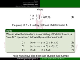
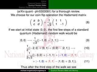
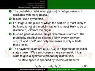
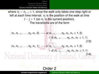
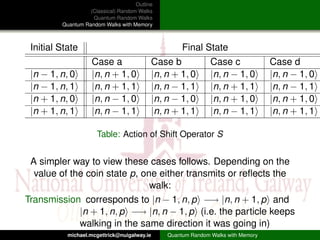
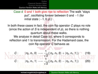
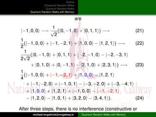
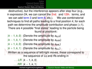
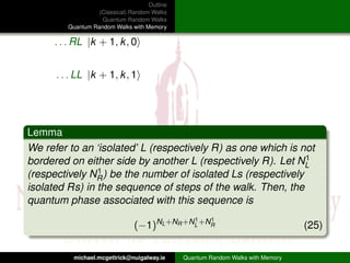
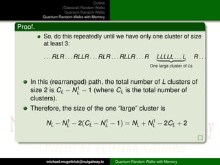
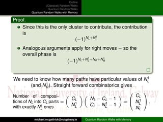
This document outlines and compares classical random walks, quantum random walks, and quantum random walks with memory. It introduces the key concepts of classical random walks on a line involving coin flips to move left or right. Quantum random walks are then described as taking place on a state space involving position and coin states, with transitions defined by unitary operators. Finally, quantum random walks with memory are discussed as generalizing the model to include memory of previous coin states.
This document discusses using hidden Markov models (HMM) for stock price prediction. HMMs can model time series data as a probabilistic finite state machine. The document explains that HMMs can handle new stock market data robustly and efficiently predict similar price patterns to past data. It provides an overview of HMM components like states, transition probabilities, and emission probabilities. The document also demonstrates building an HMM model on stock data using the RHMM package in R, including training the model with Baum-Welch and predicting state sequences with Viterbi.
This document contains slides from a lecture on pattern recognition. It discusses several topics:
- Maximum likelihood estimation and how it can be used to estimate parameters of Gaussian distributions from sample data.
- The problem of dimensionality when applying pattern recognition techniques - as the number of features or dimensions increases, classification accuracy may decrease and computational complexity increases.
- Component analysis techniques like PCA and LDA that aim to reduce dimensionality by projecting data onto a lower-dimensional space.
- An assignment involving generating an image with multiple classes, estimating class parameters with MLE, and classifying pixels with Bayesian decision theory.
This document summarizes key concepts related to Markov chains and linear algebra. It provides an example of using a transition matrix to model the probabilities of television viewers switching between two stations over time. The transition matrix allows calculating the probability vectors for future weeks through matrix multiplication. A steady-state vector can also be determined by solving the equation A*p=p, representing the long-term probabilities once the system reaches equilibrium.
DBSCAN is a density-based clustering algorithm that can find clusters of arbitrary shape. It requires two parameters: epsilon, which defines the neighborhood distance, and minimum points. It marks points as core, border or noise based on the number of points within their epsilon-neighborhood. Randomized DBSCAN improves the time complexity from O(n^2) to O(n) by randomly selecting a maximum of k points in each neighborhood to analyze rather than all points. Testing shows Randomized DBSCAN performs as well as DBSCAN in terms of accuracy while improving runtime, especially at higher data densities relative to epsilon. Future work includes analyzing accuracy in higher dimensions and combining with indexing to further improve time complexity.
probabilistic, reasoning, artificial, computer, intelligence, IOE, Sushant, Pulchowk, AI,
Statistical techniques used in practical data analysis. e.g. t-tests, ANOVA, regression, correlation;
The use of probabilistic models in psychology and linguistics
Machine learning and computational linguistics/NLP
Measure theory (in fact, almost anything involving infinite sets)
Using logic and probability to handle uncertain situation
Probability based reasoning is same as understanding directly from the knowledge that a given probability rating based on uncertainty present
This document provides an overview of Bayesian inference and filtering techniques for multi-object filtering and multi-target tracking (MOFT). It describes the problems of state estimation in dynamic systems where the state is hidden but can be partially observed. It introduces Bayesian filtering approaches which construct the posterior probability density function of the state using noisy measurements. Specific filtering techniques covered include the Kalman filter, extended Kalman filter, unscented Kalman filter, and particle filter, which make different approximations to solve the filtering problem.
This document contains lecture notes for a pattern recognition course taught by Dr. Mostafa Gadal-Haqq at Ain Shams University. The notes cover mathematical foundations of pattern recognition including probability theory, statistics, and mathematical notations. Specifically, the notes define concepts like random variables, probability distributions, expected values, variance, and conditional probability. They also provide examples of applying these concepts to problems involving events, outcomes, and data modeling. The document concludes by noting that the next lecture will cover Bayesian decision theory.
This document provides an overview of multilayer perceptrons (MLPs) and the backpropagation algorithm. It defines MLPs as neural networks with multiple hidden layers that can solve nonlinear problems. The backpropagation algorithm is introduced as a method for training MLPs by propagating error signals backward from the output to inner layers. Key steps include calculating the error at each neuron, determining the gradient to update weights, and using this to minimize overall network error through iterative weight adjustment.
Coursera Machine Learning by Andrew NG 강의를 들으면서, 궁금했던 내용을 중심으로 정리.
내가 궁금했던건, 데이터를 분류하는 Decision boundary를 만들때...
- 왜 가중치(W)와 decision boundary가 직교해야 하는지?
- margin은 어떻게 계산하는지?
- margin은 어떻게 최대화 할 수 있는지?
- 실제로 margin을 최대화 하는 과정의 수식은 어떤지?
- 비선형 decision boundary를 찾기 위해서 어떻게 kernel을 이용하는지?...
http://blog.naver.com/freepsw/221032379891
This document provides an overview of particle filtering and sampling algorithms. It discusses key concepts like Bayesian estimation, Monte Carlo integration methods, the particle filter, and sampling algorithms. The particle filter approximates probabilities with weighted samples to estimate states in nonlinear, non-Gaussian systems. It performs recursive Bayesian filtering by predicting particle states and updating their weights based on new observations. While powerful, particle filters have high computational complexity and it can be difficult to determine the optimal number of particles.
The document discusses leveraged Gaussian processes and their applications to learning from demonstration and uncertainty modeling. It introduces key concepts such as Gaussian processes, leveraged Gaussian processes, leveraged optimization, and uncertainty modeling in deep learning. It also discusses several applications including using both positive and negative demonstrations, learning from demonstration, and incorporating data with mixed qualities without explicit labeling.
The document discusses singular value decomposition (SVD), which is a way to decompose a matrix A into three matrices: A = UΣV^T. U and V are orthogonal matrices, and Σ is a diagonal matrix containing the singular values of A. SVD can be used to perform dimensionality reduction by approximating A using only the top k singular values/vectors in Σ, U, and V^T. This reduces the number of parameters needed to represent A while retaining most of its information.
Gradient Steepest method application on Griewank Function Imane Haf
The document discusses applying the gradient method to minimize the Griewank test function. It outlines the gradient method algorithm, shows simulation results for different starting points that converge in few iterations, and improvements made to ensure the algorithm finds the global minimum regardless of starting point by continuing to search after reaching local minima. The conclusions state the gradient method performs well locally but extensions were needed to locate the true global minimum for the Griewank function.
What if there’s a better way to run more complex tests and gain results faster? Joni explains the wonderful world of multi-armed bandit experiments.
About Joni
Joni Turunen is a Senior Developer at FROSMO currently working in the Product Team. He has vast experience with different frontend & backend technologies. With his 8 year history in the company he knows Frosmo's software inside out.
Multivariate Linear Regression involves modeling the relationship between a dependent variable (Y) and multiple independent variables (X1, X2, etc.). This improves the ability to predict and explain variation in Y compared to a single variable model. Key points include:
- Coefficients now represent the marginal change in Y from a one unit change in a given X, while holding other X's constant.
- Multicollinearity occurs when X's are correlated, making coefficient estimates less reliable.
- Remedies include dropping variables, combining variables, or determining the correct specification from subject matter experts.
Bayes theorem and Naive Bayes algorithmLuis Serrano
The document discusses the Naive Bayes classifier algorithm for spam detection. It shows how the algorithm calculates the probability that an email is spam based on the presence of words like "buy" and "cheap". It begins with small amounts of sample data that indicate high spam probabilities for individual words. However, it then collects more representative sample data that shows the words actually occur independently, leading to a lower calculated spam probability when both words are present. The document is an example walkthrough of how Naive Bayes modeling works for spam filtering.
Prediciting restaurant and popularity based on Yelp Dataset project reportALIN BABU
This document discusses a machine learning project that aims to predict restaurant ratings and popularity changes on Yelp using logistic regression, naive bayes, and multinomial naive bayes models. The project uses a Yelp dataset containing 20000 restaurant reviews to evaluate these algorithms. Logistic regression performed slightly better than the other methods at predicting ratings, though all methods' predictions still require improvement. More data and tailored methods may enhance predictions.
This document provides an introduction to ensemble learning techniques. It defines ensemble learning as combining the predictions of multiple machine learning models. The main ensemble methods described are bagging, boosting, and voting. Bagging involves training models on random subsets of data and combining results by majority vote. Boosting iteratively trains models to focus on misclassified examples from previous models. Voting simply averages the predictions of different model types. The document discusses how these techniques are implemented in scikit-learn and provides examples of decision tree bagging on the Iris dataset.
This document provides a summary of Lecture 2 on Markov Decision Processes. It begins with an introduction to Markov processes and their properties. Markov decision processes are then introduced as Markov processes where decisions can be made. The key components of MDPs are defined, including states, actions, transition probabilities, rewards and policies. Value functions are also introduced, which estimate the long-term value or return of states and state-action pairs. Examples are provided throughout to illustrate these concepts.
- The thesis studies numerical methods for stochastic partial differential equations (SPDEs) subject to generalized Levy noise.
- It develops both deterministic methods using the Fokker-Planck equation and probabilistic methods like polynomial chaos.
- Key contributions include developing adaptive multi-element polynomial chaos for discrete measures, comparing approaches to construct orthogonal polynomials over discrete measures, and improving efficiency and accuracy through adaptive integration meshes and sparse grids.
The document discusses Taylor series and how they can be used to approximate functions. It provides an example of using Taylor series to approximate the cosine function. Specifically:
1) It derives the Taylor series for the cosine function centered at x=0.
2) It shows that this Taylor series converges absolutely for all x.
3) It demonstrates that the Taylor series equals the cosine function everywhere based on properties of the remainder term.
4) It provides an example of using the Taylor series to approximate cos(0.1) to within 10^-7, the accuracy of a calculator display.
This document discusses a technique called "data smashing" for zero-knowledge feature-free anomaly detection in data. Data smashing involves quantizing, inverting, and comparing signals to detect anomalies without extracting or using features from the data. It allows detection of deviations from normal patterns in an unlabeled dataset in a way that preserves privacy and limits assumptions about the data's features or generation process.
Lesson31 Higher Dimensional First Order Difference Equations SlidesMatthew Leingang
This document summarizes a lesson on higher dimensional difference equations. It discusses:
1) Linear systems described by equations of the form y(k+1) = Ay(k) and their solutions involving eigenvalues and eigenvectors of A.
2) Qualitative analysis of diagonal systems based on the magnitudes of the eigenvalues determining behaviors like attraction, repulsion, or saddle points.
3) The nonlinear case where equilibria y* are found as solutions to g(y*)=y* and stability is determined by eigenvalues of the Jacobian matrix Dg(y*) evaluated at the equilibria.
The document discusses quaternions and their applications. It begins by providing a brief history of quaternions, defined by Sir William Rowan Hamilton in 1843. Quaternions represent rotations and orientations in 3D space and are used in computer graphics, control theory, physics, and other fields due to advantages like avoiding gimbal lock. The document then covers details of quaternion operations like addition, multiplication, and rotation representations. It provides examples of using quaternions to represent and perform rotations in three dimensions.
This document discusses cryptography and attacks on cryptosystems. It begins with an introduction to classical ciphers like the Caesar cipher and transposition cipher. It then covers the mathematics behind public key cryptography schemes like RSA, including number theory concepts like modulo arithmetic, discrete logarithms, and the Chinese Remainder Theorem. The document discusses the computational basis for RSA security in factoring large numbers and discusses different types of attacks on RSA like timing attacks, implementation attacks, and mathematical attacks using lattice basis reduction. It concludes with recommendations for building a secure RSA system, such as using large random paddings, large secret exponents, and generating strong prime numbers.
The document summarizes solutions to problems from an ICPC competition. It discusses solutions to 8 problems:
1. Problem B on squeezing cylinders can be solved in O(N2) time by moving cylinders from left to right using Pythagorean theorem.
2. Problem C on sibling rivalry can be solved in O(n3) time using matrix multiplication to track reachable vertices, and iterating to minimize/maximize number of turns.
3. Problem D on wall clocks can be solved greedily in O(n2) time by sorting interval positions and placing clocks at rightmost positions.
4. Problem K on the min-max distance game can be solved by binary searching the distance t and
This document introduces hierarchical quantum walks, which generalize standard quantum walks by incorporating memory. It discusses:
1) Quantum walks with memory of order p, where the direction depends on the previous p positions.
2) Reversible and irreversible higher order walks, where reversibility depends on the boolean function used.
3) Hierarchical quantum walks, where the order is itself a Markov process, allowing dynamic variation in memory length. This adds multiple levels of hierarchy to the walk.
The document discusses techniques for uncertainty propagation and constructing surrogate models. It describes Monte Carlo sampling, analytic techniques, and perturbation techniques for propagating uncertainties in nonlinear models. It also discusses constructing surrogate models such as polynomial, Kriging, and Gaussian process models to approximate computationally expensive discretized partial differential equation models for applications such as Bayesian calibration and design. The document provides an example of constructing a quadratic surrogate model to approximate the response of a heat equation model.
In the last decades, a new model of computation based on quantum mechanics has gained attention in the computer science community. We give an introduction to this model starting from the basics, with no prerequisites. Then, with the help of some simple examples, we see why quantum computers outperform standard ones in certain tasks. We then move to the topic of quantum entanglement and show how sharing quantum information can create a strong provable correlation among distant parties. With this basic understanding of quantum computation and quantum entanglement, we can already illustrate two interesting cryptographic protocols: quantum key distribution and position verification. Both perform classically impossible tasks: the first allows to detect an intruder intercepting a secret communication, while the second allows certifying somebody's GPS location.
This document discusses Bayesian variable selection methods for regression models. It begins by reviewing traditional ANOVA tables and their limitations for modern applications with many variables, such as GWAS studies. It then introduces Bayesian approaches using priors to perform variable selection by building it into the regression model. Several variable selection methods are described that use different prior distributions, such as slab and spike priors, the stochastic search variable selection (SSVS) method, and the normal-exponential-gamma (NEG) distribution. The document discusses how these methods can be implemented using MCMC sampling and compares their performance. It also discusses some extensions like using random effects and polynomial terms.
The document summarizes geometric and harmonic series. It defines geometric series as having the form ΣCrk where C and r are fixed numbers, and each term is r times the previous term. It provides a theorem showing that a geometric series converges to 1/(1-r) if |r|<1 and diverges if |r|≥1. The harmonic series Σ1/k, where each term is the reciprocal of the term number, is shown to diverge using a grouping argument where the partial sums exceed n/2.
This document provides a summary of spatial data modeling and analysis techniques. It begins with an outline of the topics to be covered, including additive statistical models for spatial data, spatial covariance functions, the multivariate normal distribution, kriging for prediction and uncertainty, and the likelihood function for parameter estimation. It then introduces the key concepts and equations for modeling spatial processes as Gaussian random fields with specified covariance functions. Examples are given of commonly used covariance functions and the types of random surfaces they generate. Kriging is described as a best linear unbiased prediction technique that uses a spatial covariance function and observations to make predictions at unknown locations. The document concludes with examples of parameter estimation via maximum likelihood and using the fitted model to make predictions and conditional simulations
International Conference on Monte Carlo techniques
Closing conference of thematic cycle
Paris July 5-8th 2016
Campus les cordeliers
Jere Koskela's slides
This document discusses clustering random walk time series. It introduces the concept of clustering and discusses challenges in clustering time series, such as how to define a distance between dependent random variables. It proposes using the copula transform and empirical copula transform to map time series to uniform distributions before calculating distances. The hierarchical block model for nested data partitions is presented. Experimental results show the proposed distances perform well in recovering the nested partitions on both synthetic hierarchical block model data and real credit default swap time series data. Consistency of clustering algorithms is defined in relation to recovering the hierarchical block model partitions.
This document provides an overview of Markov chain Monte Carlo (MCMC) methods. It begins with motivations for using MCMC, such as dealing with latent variable models where the likelihood function is intractable. It then covers random variable generation techniques before introducing the key MCMC algorithms: the Metropolis-Hastings algorithm and the Gibbs sampler. The document outlines the remaining topics to be covered, which include Monte Carlo integration, notions of Markov chains, and further advanced topics.
This document presents a summary of a talk on building a harmonic analytic theory for the Gaussian measure and the Ornstein-Uhlenbeck operator. It discusses how the Gaussian measure is non-doubling but satisfies a local doubling property. It introduces Gaussian cones and shows how they allow proving maximal function estimates for the Ornstein-Uhlenbeck semigroup in a similar way as for the heat semigroup. The talk outlines estimates for the Mehler kernel of the Ornstein-Uhlenbeck semigroup and combines them to obtain boundedness of the maximal function.
Monte Caro Simualtions, Sampling and Markov Chain Monte CarloXin-She Yang
Pseudorandom
Pseudorandom The document discusses Monte Carlo methods and Markov chain Monte Carlo (MCMC). It provides examples of using Monte Carlo simulations to estimate pi and solve Buffon's needle problem. It also discusses random walks in Markov chains, the PageRank algorithm used by Google, and challenges with high-dimensional integrals and distributions that do not have a closed-form inverse. MCMC methods are presented as a way to address these challenges.
Regularized Estimation of Spatial PatternsWen-Ting Wang
In climate and atmospheric research, many phenomena involve more than one meteorological spatial processes covarying in space. To understand how one process is affected by another, maximum covariance analysis (MCA) is commonly applied. However, the patterns obtained from MCA may sometimes be difficult to interpret. In this paper, we propose a regularization approach to promote spatial features in dominant coupled patterns by introducing smoothness and sparseness penalties while accounting for their orthogonalities. We develop an efficient algorithm to solve the resulting optimization problem by using the alternating direction method of multipliers. The effectiveness of the proposed method is illustrated by several numerical examples, including an application to study how precipitations in east Africa are affected by sea surface temperatures in the Indian Ocean.
AVRUPA KONUTLARI ESENTEPE - ENGLISH - Listing TurkeyListing Turkey
Looking for a new home in Istanbul? Look no further than Avrupa Konutlari Esentepe! Our beautifully designed homes provide the perfect blend of luxury and comfort, making them the perfect choice for anyone looking for a high-quality home in the city.
With a wide range of apartment types available, from 1+1 to 4+1, we have something to suit every need and budget. Each apartment is designed with attention to detail and features spacious and bright living areas, making them the perfect place to relax and unwind after a long day.
One of the things that sets Avrupa Konutlari Esentepe apart from other developments is our focus on creating a community that is both comfortable and convenient. Our homes are surrounded by lush green spaces, perfect for enjoying a peaceful stroll or having a picnic with friends and family. Additionally, our complex includes a variety of social and recreational amenities, such as swimming pools, sports fields, and playgrounds, making it easy for residents to stay active and socialize with their neighbors.
https://listingturkey.com/property/avrupa-konutlari-esentepe/
The SVN® organization shares a portion of their new weekly listings via their SVN Live® Weekly Property Broadcast. Visit https://svn.com/svn-live/ if you would like to attend our weekly call, which we open up to the brokerage community.
BEST FARMLAND FOR SALE | FARM PLOTS NEAR BANGALORE | KANAKAPURA | CHICKKABALP...knox groups real estate
welcome to knox groups real estate company in Bangalore. best farm land for sale near Bangalore and madhugiri . Managed farmland near Kanakapura and Chickkabalapur get know more details about the projects .Knox groups is a leading real estate company dedicated to helping individuals and businesses navigate the dynamic real estate market. With our extensive knowledge, experience, and commitment to excellence, we deliver exceptional results for our clients. Discover the perfect foundation for your agricultural aspirations with KNOX Groups' prime farm lands. These aren't just plots; they're the fertile grounds where vibrant crops flourish, livestock thrives, and unique agricultural ventures come to life. At KNOX, we go beyond selling land we curate sustainable ecosystems, ensuring that your journey toward agricultural success is seamless and prosperous.
Stark Builders: Where Quality Meets Craftsmanship!shuilykhatunnil
At Stark Builders our vision is to redefine the renovation experience by combining both stunning design and high quality construction skills. We believe that by delivering both these key aspects together we are able to achieve incredible results for our clients and ensure every project reflects their vision and enhances their lifestyle.
Although we are not all related by blood we have created a team of highly professional and hardworking individuals who share the common goal of delivering beautiful and functional renovated spaces. Our tight nit team are able to work together in a way where we pour our passion into each and every project as we have a love for what we do. Building is our life.
Living in an UBER World - June '24 Sales MeetingTom Blefko
June 2024 Lancaster County Sales Meeting for Berkshire Hathaway HomeServices Homesale Realty covering the following topics: 1. VA Suspends Buyer Agent Payment Plan (article), 2. Frequently Used Terms in title, 3. Zillow Showcase Overview, 4. QuickBuy commission promotion, 5. Documenting Cooperative Compensation, 6. NAR's Code of Ethics - Mass Media Solicitations, 7. Is it really cheaper to rent? 8. Do's and Don't's when Terminating the Agreement of Sale, 9. Living in an UBER World
Dholera Smart City Latest Development Status 2024.pdfShivgan Infratech
Explore the latest development status of Dholera Smart City in 2024. Discover the progress, infrastructure, and future plans of India's first greenfield smart city.
The SVN® organization shares a portion of their new weekly listings via their SVN Live® Weekly Property Broadcast. Visit https://svn.com/svn-live/ if you would like to attend our weekly call, which we open up to the brokerage community.
1. Outline
(Classical) Random Walks
Quantum Random Walks
Quantum Random Walks with Memory
Michael Mc Gettrick
michael.mcgettrick@nuigalway.ie
The De Brún Centre for Computational Algebra, School of Mathematics, The
National University of Ireland, Galway
Winter School on Quantum Information, Maynooth
January 2010
michael.mcgettrick@nuigalway.ie Quantum Random Walks with Memory
2. Outline
(Classical) Random Walks
Quantum Random Walks
Quantum Random Walks with Memory
Outline
1 Outline
2 (Classical) Random Walks
3 Quantum Random Walks
The Hadamard Walk
4 Quantum Random Walks with Memory
Generalized memory
Order 2
Order 2 Hadamard walk
Amplitudes
Sketch of Combinatorial caculations
michael.mcgettrick@nuigalway.ie Quantum Random Walks with Memory
3. Outline
(Classical) Random Walks
Quantum Random Walks
Quantum Random Walks with Memory
A classical random walk can be defined by specifying
1 States: |n for n ∈ Z
2 Allowed transitions:
|n − 1 a left move
|n → or
|n + 1 a right move
3 An initial state: |0
4 Rule(s) to carry out the transitions: In our case we toss a
(fair) coin , and move left or right with equal probability
(0.5).
michael.mcgettrick@nuigalway.ie Quantum Random Walks with Memory
4. Outline
(Classical) Random Walks
Quantum Random Walks
Quantum Random Walks with Memory
This defines a 1 dimensional random walk, sometimes known
as the “drunk man’s walk”, which is well understood in
mathematics and computer science. Let us denote by pc (n, k )
the probability of finding the particle at position k in an n step
walk (−n ≤ k ≤ n). Some of its properties are
1 The probability distribution is Gaussian (plot of pc (n, k )
against k ).
2 For an odd (even) number of steps, the particle can only
finish at an odd (even) integer position: pc (n, k ) = 0 unless
n mod 2 = k mod 2
3 The maximum probability is always at the origin (for an
even number of steps in the walk): pc (n, 0) > pc (n, k ) for
even n and even k = 0.
4 For an infinitely long walk, the probability of finding the
particle at any fixed point goes to zero:
limn→∞ pc (n, k ) = 0.
michael.mcgettrick@nuigalway.ie Quantum Random Walks with Memory
5. Outline
(Classical) Random Walks
Quantum Random Walks
Quantum Random Walks with Memory
Example: A short classical walk
In a 3 step walk, starting at |0 , what is the probability of finding
the particle at the point |−1 ?
We denote by L(R) a left (right) step respectively.
Possible paths that terminate at |−1 are LLR, LRL and
RLL, i.e. those paths with precisely 1 right step and 2 left
steps. So there are 3 possible paths.
Total number of possible paths is 23 = 8.
So the probability is 3/8 = 0.375.
So, how do we calculate the probabilities?
Physicist (Feynman) Path Integral.
Statistician Summation over Outcomes.
Let us denote by NL the number of left steps and NR the
number of right steps. Of course, fixing NL and NR fixes k and
michael.mcgettrick@nuigalway.ie Quantum Random Walks with Memory
6. Outline
(Classical) Random Walks
Quantum Random Walks
Quantum Random Walks with Memory
n, and vice versa: The equations are
NR + NL = n
NR − NL = k
We have an easy closed form solution for the probabilities
pc (n, k ): For a fixed NL and NR ,
n! n!
n
= = pc (n, k )
NL !NR !2 ((n − k )/2)!((n + k )/2)!2n
We can tabulate the probabilities for the first few iterations:
michael.mcgettrick@nuigalway.ie Quantum Random Walks with Memory
7. Outline
(Classical) Random Walks
Quantum Random Walks
Quantum Random Walks with Memory
Number of steps
position 0 1 2 3 4
4 0 0 0 0 0.0625
3 0 0 0 0.125 0
2 0 0 0.25 0 0.0625
1 0 0.5 0 0.375 0
0 1 0 0.5 0 0.0375
−1 0 0.5 0 0.375 0
−2 0 0 0.25 0 0.0625
−3 0 0 0 0.125 0
−4 0 0 0 0 0.0625
michael.mcgettrick@nuigalway.ie Quantum Random Walks with Memory
8. Outline
(Classical) Random Walks
Quantum Random Walks
Quantum Random Walks with Memory
Figure: Probability Distribution after 100 steps
michael.mcgettrick@nuigalway.ie Quantum Random Walks with Memory
9. Outline
(Classical) Random Walks
Quantum Random Walks
Quantum Random Walks with Memory
One Dimensional Discrete Quantum Walks (also known as
Quantum Markov Chains) take place on the State Space
spanned by vectors
|n, p (1)
where n ∈ Z (the integers) and p ∈ {0, 1} is a boolean variable.
p is often called the ‘coin’ state or the chirality, with
0 ≡ spin up
1 ≡ spin down
We can view p as the “quantum part” of the walk, while n is the
“classical part”.
One step of the walk is given by the transitions
|n, 0 −→ a |n − 1, 0 + b |n + 1, 1 (2)
|n, 1 −→ c |n − 1, 0 + d |n + 1, 1 (3)
michael.mcgettrick@nuigalway.ie Quantum Random Walks with Memory
10. Outline
(Classical) Random Walks
Quantum Random Walks
Quantum Random Walks with Memory
where
a b
∈ SU(2), (4)
c d
the group of 2 × 2 unitary matrices of determinant 1.
Aside
We can view the transitions as consisting of 2 distinct steps, a
“coin flip” operation C followed by a shift operation S:
C: |n, 0 −→ a |n, 0 + b |n, 1 (5)
C: |n, 1 −→ c |n, 0 + d |n, 1 (6)
S: |n, p −→ |n ± 1, p (7)
These walks have also been well studied: See Kempe
michael.mcgettrick@nuigalway.ie Quantum Random Walks with Memory
11. Outline
(Classical) Random Walks
Quantum Random Walks
Quantum Random Walks with Memory
(arXiv:quant−ph/0303081) for a thorough review.
We choose for our coin flip operation the Hadamard matrix
a b 1 1 1
=√ (8)
c d 2 1 −1
If we start at initial state |0, 0 , the first few steps of a standard
quantum (Hadamard) random walk would be
1
|0, 0 −→ √ (|−1, 0 + |1, 1 ) −→ (9)
2
1
(|−2, 0 + |0, 1 + |0, 0 − |2, 1 ) −→ (10)
2
1
√ (|−3, 0 + |−1, 1 + |−1, 0 − |1, 1
2 2
+ |−1, 0 + |1, 1 − |1, 0 + |3, 1 ). (11)
Thus after the third step of the walk we see
michael.mcgettrick@nuigalway.ie Quantum Random Walks with Memory
12. Outline
(Classical) Random Walks
Quantum Random Walks
Quantum Random Walks with Memory
destructive interference (cancellation of 4th. and 6th. terms)
constructive interference (addition of 3rd. and 5th. terms)
which are features that do not exist in the classical case.
The calculation of pq (n, k ) proceeds by again looking at all
paths that lead to a particular position k , but this time, since we
are in the quantum domain:
√
We calculate firstly amplitudes − so we have a 1/ 2 factor
added at every step, and final probabilities are amplitudes
squared (in our examples, with the Hadamard walk there
are no imaginary numbers).
There are also phases that we must take account of in our
amplitude calculations.
In particular, note that the phase −1 from the Hadamard matrix
arises every time, in a particular path, we follow a right step by
another right step.
michael.mcgettrick@nuigalway.ie Quantum Random Walks with Memory
13. Outline
(Classical) Random Walks
Quantum Random Walks
Quantum Random Walks with Memory
Brun, Carteret & Ambainis (arXiv:quant−ph/0210161) have
calculated explicitly (using combinatorial techniques) the
amplitudes:
Amplitude for final state |k , 0
M
1 NL − 1 NR
√ (−1)NL −C
2n C−1 C−1
C=1
Amplitude for final state |k , 1
M
1 NL − 1 NR
√ (−1)NL −C
2n C−1 C
C=1
where M has value NL for k ≥ 0 and value NR + 1 otherwise.
The analyses of Kempe (and others) show that for the quantum
(Hadamard) random walk with initial state |0, 0
michael.mcgettrick@nuigalway.ie Quantum Random Walks with Memory
14. Outline
(Classical) Random Walks
Quantum Random Walks
Quantum Random Walks with Memory
1 The probability distribution pq (n, k ) is not gaussian − it
oscillates with many peaks.
2 It is not even symmetric.
3 For large n, the place at which the particle is most likely to
be found is √ at the origin: rather it is most likely to be at
not
distance n/ 2 from the origin.
4 In some general sense, the particle “travels further”: The
probability distribution is spread fairly evenly between
√ √
−n/ 2 and n/ 2, and only decreases rapidly outside
these limits.
5 The asymmetric nature of pq (n, k ) is a figment of the initial
state chosen: We can choose a more symmetric initial
state to give a symmetric probability distribution.
The state space is spanned by vectors of the form
|nr , nr −1 , . . . , n2 , n1 , p (12)
michael.mcgettrick@nuigalway.ie Quantum Random Walks with Memory
15. Outline
(Classical) Random Walks
Quantum Random Walks
Quantum Random Walks with Memory
where nj = nj−1 ± 1, since the walk only takes one step right or
left at each time interval. nj is the position of the walk at time
t − j + 1 (so n1 is the current position).
The transitions are of the form
|nr , nr −1 , . . . , n2 , n1 , 0 −→ a |nr −1 , . . . , n2 , n1 , n1 ± 1, 0
+ b |nr −1 , . . . , n2 , n1 , n1 ± 1, 1
(13)
|nr , nr −1 , . . . , n2 , n1 , 1 −→ c |nr −1 , . . . , n2 , n1 , n1 ± 1, 0
+ d |nr −1 , . . . , n2 , n1 , n1 ± 1, 1
(14)
Order 2
michael.mcgettrick@nuigalway.ie Quantum Random Walks with Memory
16. Outline
(Classical) Random Walks
Quantum Random Walks
Quantum Random Walks with Memory
The state space is composed of the families of vectors
|n − 1, n, 0 , |n − 1, n, 1 , |n + 1, n, 0 , |n + 1, n, 1
(15)
for n ∈ Z . For obvious reasons, we call
|n − 1, n, p a right mover
|n + 1, n, p a left mover
As before, we can split the transitions into two steps, a “coin
flip” operator C and a “shift” operator S:
C: |n2 , n1 , 0 −→ a |n2 , n1 , 0 + b |n2 , n1 , 1 (16)
C: |n2 , n1 , 1 −→ c |n2 , n1 , 0 + d |n2 , n1 , 1 (17)
S: |n2 , n1 , p −→ |n1 , n1 ± 1, p (18)
To construct a unitary transition on the states, our possibilities
are
michael.mcgettrick@nuigalway.ie Quantum Random Walks with Memory
17. Outline
(Classical) Random Walks
Quantum Random Walks
Quantum Random Walks with Memory
Initial State Final State
Case a Case b Case c Case d
|n − 1, n, 0 |n, n + 1, 0 |n, n + 1, 0 |n, n − 1, 0 |n, n − 1, 0
|n − 1, n, 1 |n, n + 1, 1 |n, n − 1, 1 |n, n + 1, 1 |n, n − 1, 1
|n + 1, n, 0 |n, n − 1, 0 |n, n − 1, 0 |n, n + 1, 0 |n, n + 1, 0
|n + 1, n, 1 |n, n − 1, 1 |n, n + 1, 1 |n, n − 1, 1 |n, n + 1, 1
Table: Action of Shift Operator S
A simpler way to view these cases follows. Depending on the
value of the coin state p, one either transmits or reflects the
walk:
Transmission corresponds to |n − 1, n, p −→ |n, n + 1, p and
|n + 1, n, p −→ |n, n − 1, p (i.e. the particle keeps
walking in the same direction it was going in)
michael.mcgettrick@nuigalway.ie Quantum Random Walks with Memory
18. Outline
(Classical) Random Walks
Quantum Random Walks
Quantum Random Walks with Memory
Reflection corresponds to |n − 1, n, p −→ |n, n − 1, p and
|n + 1, n, p −→ |n, n + 1, p (i.e. the particle
changes direction)
so we can re draw the table as
Value of p Action of S
Case a Case b Case c Case d
0 Transmit Transmit Reflect Reflect
1 Transmit Reflect Transmit Reflect
Table: Action of Shift Operator S
Case a 0 and 1 both give rise to transmission This does
not give an interesting walk: particle moves
uniformly in one direction. For an initial state which
is a superposition of left and right movers, the walk
progresses simultaneously right and left.
michael.mcgettrick@nuigalway.ie Quantum Random Walks with Memory
19. Outline
(Classical) Random Walks
Quantum Random Walks
Quantum Random Walks with Memory
Case d 0 and 1 both give rise to reflection The walk “stays
put”, oscillating forever between 0 and −1 (for
initial state |−1, 0, p )
In both these cases in fact, the coin flip operator C plays no role
(since the action of S is independent of p), so there is nothing
quantum about these walks.
We analyse in detail Case (c), where 0 corresponds to
reflection and 1 to transmission. For the Hadamard case, the
coin flip operator C behaves as
1
C: |n2 , n1 , 0 −→ √ (|n2 , n1 , 0 + |n2 , n1 , 1 ) (19)
2
1
C: |n2 , n1 , 1 −→ √ (|n2 , n1 , 0 − |n2 , n1 , 1 ) (20)
2
michael.mcgettrick@nuigalway.ie Quantum Random Walks with Memory
20. Outline
(Classical) Random Walks
Quantum Random Walks
Quantum Random Walks with Memory
Aside: Classical Order 2 Random Walk
It should be clear that the classical order 2 random walk
corresponding to our quantum order 2 Hadamard walk behaves
exactly like a standard (order 1) classical walk.
Classical Order 1 0 always means move left (e.g. ) and 1
always means move right.
Classical Order 2 0 means reflect and 1 means transmit: So
e.g. 0 will sometimes mean “move left” and
sometimes “move right”, but always 1 will mean to
move in the opposite direction to 0.
The first few steps of the Order 2 Hadamard walk for case (c)
michael.mcgettrick@nuigalway.ie Quantum Random Walks with Memory
22. Outline
(Classical) Random Walks
Quantum Random Walks
Quantum Random Walks with Memory
destructive), but the interference appears after step four (e.g.,
in expression 24, we can cancel the 2nd. and 12th. terms, and
we can add term 3 and term 9, etc.). We use combinatorial
techniques to find all paths leading to a final position k ; for each
path we determine the amplitude contribution and phase (±1).
There are 4 possible “final states” leading to the particle being
found at positionk :
|k − 1, k , 0 (Denote the amplitude by akLR )
|k − 1, k , 1 (Denote the amplitude by akRR )
|k + 1, k , 0 (Denote the amplitude by akRL )
|k + 1, k , 1 (Denote the amplitude by akLL )
Written as a sequence of left/right moves, these correspond to
the sequence of Ls and Rs ending in
. . . LR |k − 1, k , 0
. . . RR |k − 1, k , 1
michael.mcgettrick@nuigalway.ie Quantum Random Walks with Memory
23. Outline
(Classical) Random Walks
Quantum Random Walks
Quantum Random Walks with Memory
. . . RL |k + 1, k , 0
. . . LL |k + 1, k , 1
Lemma
We refer to an ‘isolated’ L (respectively R) as one which is not
bordered on either side by another L (respectively R). Let NL 1
(respectively NR1 ) be the number of isolated Ls (respectively
isolated Rs) in the sequence of steps of the walk. Then, the
quantum phase associated with this sequence is
1 1
(−1)NL +NR +NL +NR (25)
michael.mcgettrick@nuigalway.ie Quantum Random Walks with Memory
24. Outline
(Classical) Random Walks
Quantum Random Walks
Quantum Random Walks with Memory
Proof.
We analyze firstly the contribution of clusters of Ls.
Clusters of various size contribute as follows:
Cluster
L LL LLL LLLL LLLLL LLLLLL
Phase Contribution + + - + - +
The −1 phase comes from a transmission followed by
another transmission. So the cluster of 3 Ls is the first to
contribute.
For j > 2 a cluster of j Ls gives a contribution of (−1)j .
For clusters of size at least 3:
Moving an L from one cluster to another does not change
overall phase contribution.
michael.mcgettrick@nuigalway.ie Quantum Random Walks with Memory
25. Outline
(Classical) Random Walks
Quantum Random Walks
Quantum Random Walks with Memory
Proof.
So, do this repeatedly until we have only one cluster of size
at least 3:
. . . RLR . . . RLLR . . . RLR . . . RLLR . . . R LLLLL . . . L R ...
One large cluster of Ls
In this (rearranged) path, the total number of L clusters of
1
size 2 is CL − NL − 1 (where CL is the total number of
clusters).
Therefore, the size of the one “large” cluster is
1 1 1
NL − NL − 2(CL − NL − 1) = NL + NL − 2CL + 2
michael.mcgettrick@nuigalway.ie Quantum Random Walks with Memory
26. Outline
(Classical) Random Walks
Quantum Random Walks
Quantum Random Walks with Memory
Proof.
Since this is the only cluster to contribute, the contribution
is
1
(−1)NL +NL
Analogous arguments apply for right moves − so the
overall phase is
1 1
(−1)NL +NL +NR +NR
We need to know how many paths have particular values of NL 1
(and NR 1 ). Straight forward combinatorics gives
Number of composi- CL
CL NL − CL − 1 1
tions of NL into CL parts = 1 1 = NL .
1
with exactly NL ones NL CL − NL − 1
NL
michael.mcgettrick@nuigalway.ie Quantum Random Walks with Memory
27. Outline
(Classical) Random Walks
Quantum Random Walks
Quantum Random Walks with Memory
0.55
quantum
0.5
quantum
0.45
with
0.4 memory
0.35 classical
Probability
0.3
0.25
0.2
0.15
0.1
0.05
0
-10 -8 -6 -4 -2 0 2 4 6 8 10
Position
Figure: Probability Distribution after 10 steps
michael.mcgettrick@nuigalway.ie Quantum Random Walks with Memory