Downloaded 142 times


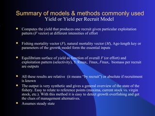

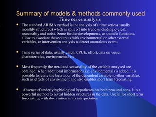
![Beverton & Holt yield per recruit model
INPUT
L∞ 28.4cm
W∞ 286gm
K 0.37
M 1.1
Lc 10.2
Lr 2.03
tc 1
tr 0
tzero -0.2
a 0.0125
b 3
a & b denote length-
weight relationship
parameters
Y/R = F*exp(-M*(tc-tr))*W∞*[1/Z – 3S/(Z+K)+ 3S2
/(Z+2K) – S3
/(Z+3K)]
Where S= exp[-K*(tc-tzero)]
Yield per recruit model
0
1
2
3
4
5
6
0 0.1 0.2 0.3 0.4 0.5 0.6 0.7 0.8 0.9 1 1.1 1.2 1.3 1.4 1.5 1.6 1.7 1.8 1.9 2
F
Y/R
Biomass per recruit curve
0.00
2.00
4.00
6.00
8.00
10.00
12.00
14.00
16.00
0 0.5 1 1.5 2 2.5
F
B/R](https://image.slidesharecdn.com/marinefishstockassessmentmodels-180124060639/85/Marine-fish-stock-assessment_models-18-320.jpg)
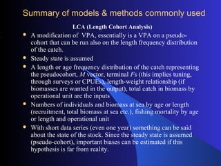
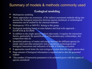
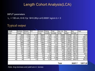
![Length Cohort Analysis(LCA)
INPUT
Length frequency data (preferably, averaged over a period of time. Say,
over 3 to 5 years)
Estimates of VBGF Growth in length parameters L∞ and K.
Instantaneous rate of natural mortality M
Estimates of parameters a and b of the l-w relationship w = a. Lb
Formulation
Let
C(L1,L2) be the numbers caught between lengths L1 and L2
N(L1) be the numbers in sea that attain length L1
N(L2) be the numbers in sea that attain length L2
H(L1,L2) = [(L∞ - L1)/(L∞ - L2) ] (M/2K)](https://image.slidesharecdn.com/marinefishstockassessmentmodels-180124060639/85/Marine-fish-stock-assessment_models-19-320.jpg)
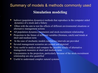
![Length Cohort analysis(LCA)
Formulae used in the analysis
N(L1) = [N(L2)*H(L1,L2) + C(L1,L2)]*H(L1,L2)
C(L1,L2) = N(L1) *(F/Z)* [ 1 – exp(-z* Δt) ]
Where Δt = (1/K) * ln [(L∞ - L1)/(L∞ - L2) ]
Calculations
Start with the last length group
Compute H for each length group H(L1,L2) = [(L∞ - L1)/(L∞ - L2) ] (M/2K)
Compute average weight for each length group as w(L1,L2)= a*[(L1+L2)/2]b
Assume a value F/Z for the last length group ( how to choose terminal F/Z ?)
Compute the numbers in sea for the last length group by dividing the catch in numbers by the terminal
F/Z
Compute, recursively, N(L1) for each length group
Compute F(L1,L2)/(Z(L1,L2) = C(L1,L2)/(N(L1) – N(L2))
Compute F(L1,L2) = M*(F(L1,L2)(/Z(L1,L2)) / (1 – (F(L1,L2)/Z(L1,L2)))
Compute Z(L1,L2) = F(L1,L2)+M
Compute average annual numbers in the sea = [N(L1) – N(L2)]/Z(L1,l2)= avg.N(L1,L2)
Catch(yield) in weight = C(L1,L2)*w(L1,L2)
Mean biomass = avg.N(L1,L2)*w(L1,L2)
Caution:: Approximation valid only when F* Δt is upto 1.2 and M* Δt upto 0.3
Output from LCA
Total mortality in each length group
Fishing mortality in each length group
Numbers in sea at the beginning of length group
Mean numbers in sea in each length group
Mean biomass(in weight) of each length group](https://image.slidesharecdn.com/marinefishstockassessmentmodels-180124060639/85/Marine-fish-stock-assessment_models-20-320.jpg)


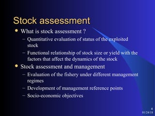
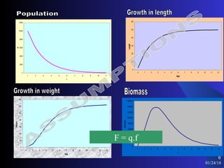
The document discusses various models and methods commonly used for marine fish stock assessment. It provides an overview of holistic or surplus production models, which analyze the relationship between effort and catch to estimate biomass and fishing mortality. Yield or yield per recruit models compute yield given exploitation patterns at different effort intensities. Virtual population analysis and cohort analysis reconstruct stock histories from catch-at-age data. Length cohort analysis is a modification of VPA that can use length frequency distributions. Time series analysis examines trends, seasonality and noise in catch or effort time series data. Ecological models account for biological interactions between species, while simulation modeling tests management actions and environmental impacts. Worked examples demonstrate length cohort analysis and yield per recruit modeling.